Unit 4
Double Integral
Recall that a single integral is something of the form

A double integral is something of the farm

Where R is called the region of integration and is a region in the (x, y) plane. The double integral gives us the volume under the surface z = f(x,y), just as a single integral gives the area under a curve
Example 1:

Solution: In this example the “inner integral” is  with y treated as a constant.


Example 2:

Solution:


Example 3: Find the volume of the solid bounded above by the plane z = 4-x-y and below by the rectangle R = {(x,y): 0 0
0 }.
}.
Solution: The volume under any surface z = f(x, y) and above a region R is given by

In our case


Example 1: Evaluate

By changing the order of integration.
Solution: The given limits are (inner) y from x to  ; (Outer) x from 0 to
  .
.
We use these to sketch the region of integration.
The given limits have inner variable y. To reverse the order of integration we use horizontal stripes. The limits in this order are
(inner) x from 0 to y; (outer) y from 0 to  .
.
So the integral becomes

We compute the inner, then the outer integrals.
Inner: 
Change of Order of Integration:

This is the case where limits are constants. But if they are variables, then by changing the order of integration, the limits of integration also changes.
A rough sketch helps in fixing the new limits of integration.
Example 1: Change the order of integration in 
Of hence evaluate the same.
Solution:

Pt. Of interaction:


Region of interaction is divided into 2 parts OAM and MAB
For region OAM:

For region MAB:


Example 2: Change the order of integration of evaluate

Solution:


Pt. Of intersection


Example 1:  is the portion of the circles of radius 2 and radius 5 cantered at the origin that line in the first quadrant.
Solution: First let’s get D terms of polar coordinates. The circle of radius 2 is given by r =2 and the circle of radius 5 is given by r =5. We want the region between the two circles, so we will have the following inequality for r.
Also, since we only want the portion that in the first quadrant, we get following range of 

Now that we’ve got these we can do the integral


Example 2:  is the unit centered at the origin.
Solution: In this case we can’t do this integral in terms of cartesian coordinates. We will however be able to do it in polar coordinates. First, the region D is defined by


In terms of polar coordinates, the integral is then,

Notice that the addition of the r is given us an integral that we can now do. Here is the work for this integral.


Example 1: Determine the area of the region bounded by
 and the y-axis.
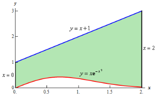
Solution: In this case the last two pieces of 8information, x =2 and the y-axis, tell us the right and left boundaries of the region. Also, recall that the y-axis is given by the line x =0. Here is the graph with the enclosed region shaded in.

Here, unlike the first example, the two curves don’t meet. Instead we rely on two vertical lines to bound the left and right sides of the region as we noted above.


Example 2: Determine the area of the region bounded

Solution: In this case the intersection points (which we’ll need eventually) are not going to be easily identified from the graph so let’s go ahead and get them now. Note that for most of these problem’s you’ll not be able to accurately identify the intersection points from the graph and so you’ll need to be able to determine them by hand. In this case we can get the intersection points by setting the two equations equal.


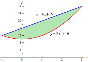
So, it looks like the two curves will intersect at x = -1 and x=3. If we need them we can get the y values corresponding to each of these by plugging the values back into either of the equations. We’ll leave it to you to verify that the coordinates of the two intersection points on the graph are(-1, 12) and (3, 28).
Note as well that if you aren’t good at graphing knowing the intersection points can help in at least getting the graph started. Here is a graph of the region.

With the graph we can now identify the upper and lower function and so we can now find the enclosed area.


Textbooks:
1. Erwin Kreyszig, Advanced Engineering Mathematics, 10/e, John Wiley & Sons, 2011.
2. B. S. Grewal, Higher Engineering Mathematics, 44/e, Khanna Publishers, 2017.
References:
1. R. K. Jain and S. R. K. Iyengar, Advanced Engineering Mathematics, 3/e, Alpha Science
International Ltd., 2002.
2. George B. Thomas, Maurice D. Weir and Joel Hass, Thomas Calculus, 13/e, Pearson
Publishers, 2013.
3. Glyn James, Advanced Modern Engineering Mathematics, 4/e, Pearson publishers, 201.
Unit 4
Double Integral
Recall that a single integral is something of the form

A double integral is something of the farm

Where R is called the region of integration and is a region in the (x, y) plane. The double integral gives us the volume under the surface z = f(x,y), just as a single integral gives the area under a curve
Example 1:

Solution: In this example the “inner integral” is  with y treated as a constant.


Example 2:

Solution:


Example 3: Find the volume of the solid bounded above by the plane z = 4-x-y and below by the rectangle R = {(x,y): 0 0
0 }.
}.
Solution: The volume under any surface z = f(x, y) and above a region R is given by

In our case


Example 1: Evaluate

By changing the order of integration.
Solution: The given limits are (inner) y from x to  ; (Outer) x from 0 to
  .
.
We use these to sketch the region of integration.
The given limits have inner variable y. To reverse the order of integration we use horizontal stripes. The limits in this order are
(inner) x from 0 to y; (outer) y from 0 to  .
.
So the integral becomes

We compute the inner, then the outer integrals.
Inner: 
Change of Order of Integration:

This is the case where limits are constants. But if they are variables, then by changing the order of integration, the limits of integration also changes.
A rough sketch helps in fixing the new limits of integration.
Example 1: Change the order of integration in 
Of hence evaluate the same.
Solution:

Pt. Of interaction:


Region of interaction is divided into 2 parts OAM and MAB
For region OAM:

For region MAB:


Example 2: Change the order of integration of evaluate

Solution:


Pt. Of intersection


Example 1:  is the portion of the circles of radius 2 and radius 5 cantered at the origin that line in the first quadrant.
Solution: First let’s get D terms of polar coordinates. The circle of radius 2 is given by r =2 and the circle of radius 5 is given by r =5. We want the region between the two circles, so we will have the following inequality for r.
Also, since we only want the portion that in the first quadrant, we get following range of 

Now that we’ve got these we can do the integral


Example 2:  is the unit centered at the origin.
Solution: In this case we can’t do this integral in terms of cartesian coordinates. We will however be able to do it in polar coordinates. First, the region D is defined by


In terms of polar coordinates, the integral is then,

Notice that the addition of the r is given us an integral that we can now do. Here is the work for this integral.


Example 1: Determine the area of the region bounded by
 and the y-axis.
Solution: In this case the last two pieces of 8information, x =2 and the y-axis, tell us the right and left boundaries of the region. Also, recall that the y-axis is given by the line x =0. Here is the graph with the enclosed region shaded in.

Here, unlike the first example, the two curves don’t meet. Instead we rely on two vertical lines to bound the left and right sides of the region as we noted above.


Example 2: Determine the area of the region bounded

Solution: In this case the intersection points (which we’ll need eventually) are not going to be easily identified from the graph so let’s go ahead and get them now. Note that for most of these problem’s you’ll not be able to accurately identify the intersection points from the graph and so you’ll need to be able to determine them by hand. In this case we can get the intersection points by setting the two equations equal.


So, it looks like the two curves will intersect at x = -1 and x=3. If we need them we can get the y values corresponding to each of these by plugging the values back into either of the equations. We’ll leave it to you to verify that the coordinates of the two intersection points on the graph are(-1, 12) and (3, 28).
Note as well that if you aren’t good at graphing knowing the intersection points can help in at least getting the graph started. Here is a graph of the region.

With the graph we can now identify the upper and lower function and so we can now find the enclosed area.


Textbooks:
1. Erwin Kreyszig, Advanced Engineering Mathematics, 10/e, John Wiley & Sons, 2011.
2. B. S. Grewal, Higher Engineering Mathematics, 44/e, Khanna Publishers, 2017.
References:
1. R. K. Jain and S. R. K. Iyengar, Advanced Engineering Mathematics, 3/e, Alpha Science
International Ltd., 2002.
2. George B. Thomas, Maurice D. Weir and Joel Hass, Thomas Calculus, 13/e, Pearson
Publishers, 2013.
3. Glyn James, Advanced Modern Engineering Mathematics, 4/e, Pearson publishers, 201.