Unit 1
Matrix operations and solving systems of linear equations
The rank of a matrix (r) can be defined as –
1. It has at least one non-zero minor of order r.
2. Every minor of A of order higher than r is zero.
Example 1: Find the rank of a matrix M by echelon form.
M = 
Solution: First we will convert the matrix M into echelon form,
M = 
Apply,  , we get
M = 
Apply  , we get
M = 
Apply 
M = 
We can see that, in this echelon form of matrix, the number of non – zero rows is 3.
So that the rank of matrix X will be 3.
Example 2: Find the rank of a matrix A by echelon form.
A = 
Solution: Convert the matrix A into echelon form,
A = 
Apply 
A = 
Apply  , we get
A = 
Apply  , we get
A = 
Apply  ,
,
A = 
Apply  ,
,
A = 
Therefore, the rank of the matrix will be 2.
Example 3: Find the rank of a matrix A by echelon form.
A = 
Solution: Transform the matrix A into echelon form, then find the rank,
We have,
A = 
Apply, 
A = 
Apply  ,
,
A = 
Apply 
A = 
Apply 
A = 
Hence the rank of the matrix will be 2.
Example 4: Find the rank of the following matrices by echelon form?
Solution: Let A = 
Applying 
A 
Applying 
A 
Applying 
A 
Applying 
A 
It is clear that minor of order 3 vanishes but minor of order 2 exists as 
Hence rank of a given matrix A is 2 denoted by 
2. 
Let A = 
Applying 

Applying 

Applying 

The minor of order 3 vanishes but minor of order 2 non zero as 
Hence the rank of matrix A is 2 denoted by 
3. 
Let A = 
Apply 

Apply 

Apply 

It is clear that the minor of order 3 vanishes whereas the minor of order 2 is non zero as 
Hence the rank of given matrix is 2 i.e. 
There are two types of linear equations-
1. Consistent
2. Inconsistent
Let’s understand about these two types of linear equations.
Consistent –
If a system of equations has one or more than one solution, it is said be consistent.
There could be unique solution or infinite solution.
For example-
A system of linear equations-
2x + 4y = 9
x + y = 5
Has unique solution,
Whereas,
A system of linear equations-
2x + y = 6
4x + 2y = 12
Has infinite solutions.
Inconsistent-
If a system of equations has no solution, then it is called inconsistent.
Consistency of a system of linear equations-
Suppose that a system of linear equations is given as-


This is the format as AX = B
Its augmented matrix is-
[A:B] = C
(1) Consistent equations-
If Rank of A = Rank of C
Here, Rank of A = Rank of C = n (no. Of unknown) – unique solution
And Rank of A = Rank of C = r, where r<n - infinite solutions
(2) Inconsistent equations-
If Rank of A ≠ Rank of C
Solution of homogeneous system of linear equations-
A system of linear equations of the form AX = O is said to be homogeneous, where A denotes the coefficients and of matrix and O denotes the null vector.
Suppose the system of homogeneous linear equations is,


It means,
AX = O
Which can be written in the form of matrix as below,

Note- A system of homogeneous linear equations always has a solution if
1. r(A) = n then there will be trivial solution, where n is the number of unknown,
2. r(A) < n , then there will be an infinite number of solution.
Example 1: Find the solution of the following homogeneous system of linear equations,


Solution: The given system of linear equations can be written in the form of matrix as follows,

Apply the elementary row transformation,


 , we get,
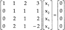

 , we get

Here r(A) = 4, so that it has trivial solution,

Example 2: Find out the value of ‘b’ in the system of homogeneous equations-
2x + y + 2z = 0
x + y + 3z = 0
4x + 3y + bz = 0
Which has
(1) Trivial solution
(2) Non-trivial solution
Solution: (1) For trivial solution, we already know that the values of x , y and z will be zero, so that ‘b’ can have any value.
Now for non-trivial solution-
(2)
Convert the system of equations into matrix form-
AX = O

Apply  Respectively , we get the following resultant matrices


For non-trivial solutions, r(A) = 2 < n
b – 8 = 0
b = 8
Solution of non-homogeneous system of linear equations-
Example-3: check whether the following system of linear equations is consistent of not.
2x + 6y = -11
6x + 20y – 6z = -3
6y – 18z = -1
Solution: Write the above system of linear equations in augmented matrix form,

Apply  , we get

Apply 

Here the rank of C is 3 and the rank of A is 2
Therefore, both ranks are not equal. So that the given system of linear equations is not consistent.
Example 4: Check the consistency and find the values of x , y and z of the following system of linear equations.
2x + 3y + 4z = 11
X + 5y + 7z = 15
3x + 11y + 13z = 25
Solution. Re-write the system of equations in augmented matrix form.
C = [A, B]
That will be,

Apply 

Now apply ,
We get,
 ~
~ ~
~
Here rank of A = 3
And rank of C = 3, so that the system of equations is consistent,
So that we can solve the equations as below,
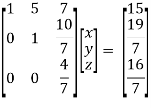
That gives,
x + 5y + 7z = 15 ……………..(1)
y + 10z/7 = 19/7 ………………(2)
4z/7 = 16/7 ………………….(3)
From eq. (3)
z = 4,
From 2,

From eq.(1), we get
x + 5(-3) + 7(4) = 15
That gives,
x = 2
Therefore the values of x , y , z are 2 , -3 , 4 respectively.
Gauss-Seidel iteration method-
Step by step method to solve the system of linear equation by using Gauss Seidal Iteration method-
Suppose,


This system can be written as after dividing it by suitable constants,


Step-1 Here put y = 0 and z = 0 and x =  in first equation
Then in second equation we put this value of x that we get the value of y.
In the third eq. We get z by using the values of x and y
Step-2: we repeat the same procedure
Example 5: solve the following system of linear equations by using Guassseidel method-
6x + y + z = 105
4x + 8y + 3z = 155
5x + 4y - 10z = 65
Solution: The above equations can be written as,
 ………………(1)
 ………………………(2)
 ………………………..(3)
Now put z = y = 0 in first eq.
We get
x = 35/2
Put x = 35/2 and z = 0 in eq. (2)
We have,

Put the values of x and y in eq. 3

Again start from eq.(1)
By putting the values of y and z
y = 85/8 and z = 13/2
We get

The process can be showed in the table format as below
Iterations | 1 | 2 | 3 | 4 |
 | 32/2=17.5 | 14.64 | 15.12 | 14.98 |
 | 85/8=10.6 | 9.62 | 10.06 | 9.98 |
 | 13/2=6.5 | 4.67 | 5.084 | 4.98 |
At the fourth iteration, we get the values of x = 14.98, y = 9.98, z = 4.98
Which are approximately equal to the actual values?
As x = 15, y = 10 and y = 5 (which are the actual values)
Example6: Solve the following system of linear equations by using Guassseidel method-
5x + 2y + z = 12
x + 4y + 2z = 15
x + 2y + 5z = 20
Solution: These equations can be written as ,
 ………………(1)
 ………………………(2)
 ………………………..(3)
Put y and z equals to 0 in eq. 1
We get,
x = 2.4
Put x = 2.4, and z = 0 in eq. 2 , we get

Put x = 2.4 and y = 3.15 in eq.(3) , we get

Again start from eq.(1), put the values of y and z , we get
 = 0.688
We repeat the process again and again,
The following table can be obtained –
Iterations | 1 | 2 | 3 | 4 | 5 |
 | 2.4 | 0.688 | 0.84416 | 0.962612 | 0.99426864 |
 | 3.15 | 2.448 | 2.09736 | 2.013237 | 2.00034144 |
 | 2.26 | 2.8832 | 2.99222 | 3.0021828 | 3.001009696 |
We see that the values are approx. Equal to exact values.
Exact values are, x = 1, y = 2, z = 3.
First, we will go through some important definitions before studying Eigen values and Eigen vectors.
1. Vector-
An ordered n – couple of numbers is called an n – vector. Thus the ‘n’ numbers x1, x2, …………xn taken in order denote the vector x. i.e. x = (x1, x2, ……., xn).
Where the numbers x1, x2, ………..,xn are called component or co – ordinates of a vector x. A vector may be written as row vector or a column vector.
If A be an mxn matrix then each row will be an n – vector & each column will be an m – vector.
2. Linear dependence-
A set of n – vectors. x1, x2, …….., xr is said to be linearly dependent if there exist scalars. k1, k2, …….,kr not all zero such that
k1 + x2k2 + …………….. + xrkr = 0 … (1)
3. Linear independence-
A set of r vectors x1, x2, ………….,xr is said to be linearly independent if there exist scalars k1, k2, …………, kr all zero such that
x1 k1 + x2 k2 + …….. + xrkr = 0
Important notes-
- Equation (1) is known as a vector equation.
- If the vector equation has non – zero solution i.e. k1, k2, ….,kr not all zero. Then the vector x1, x2, ……….xr are said to be linearly dependent.
- If the vector equation has only trivial solution i.e.
k1 = k2 = …….=kr = 0. Then the vector x1, x2, ……,xr are said to linearly independent.
4. Linear combination-
A vector x can be written in the form.
x = x1 k1 + x2 k2 + ……….+xrkr
Where k1, k2, ………….., kr are scalars, then X is called linear combination of x1, x2, ……, xr.
Results:
- A set of two or more vectors are said to be linearly dependent if at least one vector can be written as a linear combination of the other vectors.
- A set of two or more vector are said to be linearly independent then no vector can be expressed as linear combination of the other vectors.
Example1: Are the vectors  ,
,  ,
,  linearly dependent. If so, express x1 as a linear combination of the others.
Solution: Consider a vector equation,

i.e. 


Which can be written in matrix form as,


Here  & no. Of unknown 3. Hence the system has infinite solutions. Now rewrite the questions as,


Put 
 and
and


Thus 
i.e. 
i.e. 


Since F11k2, k3 not all zero. Hence  are linearly dependent.
Example 2: Examine whether the following vectors are linearly independent or not.
 and
and  .
.
Solution: Consider the vector equation,

i.e.  … (1)
… (1)


Which can be written in matrix form as,

R12

R2 – 3R1, R3 – R1


R3 + R2

Here Rank of coefficient matrix is equal to the no. Of unknowns. i.e. r = n = 3.
Hence the system has unique trivial solution.
i.e. 
i.e. vector equation (1) has only trivial solution. Hence the given vectors x1, x2, x3 are linearly independent.
Example 3: At what value of P the following vectors are linearly independent.

Solution:
Consider the vector equation.

i.e.


This is a homogeneous system of three equations in 3 unknowns and has a unique trivial solution.
If and only if Determinant of coefficient matrix is non zero.
 consider
  .
.
 .
.
i.e.


Thus for  the system has only trivial solution and Hence the vectors are linearly independent.
Note:-
If the rank of the coefficient matrix is r, it contains r linearly independent variables & the remaining vectors (if any) can be expressed as linear combination of these vectors.
Characteristic equation:-
Let A he a square matrix,  be any scalar then
  is called characteristic equation of a matrix A.
Note:
Let a be a square matrix and ‘ ’ be any scalar then,
1)  is called characteristic matrix
2)  is called characteristic polynomial.
The roots of a characteristic equations are known as characteristic root or latent roots, Eigen values or proper values of a matrix A.
Eigen vector:-
Suppose  be an Eigen value of a matrix A. Then
  a non – zero vector x1 such that.
 … (1)
… (1)
Such a vector ‘x1’ is called as Eigen vector corresponding to the Eigen value  .
.
Properties of Eigen values:-
- Then sum of the Eigen values of a matrix A is equal to sum of the diagonal elements of a matrix A.
- The product of all Eigen values of a matrix A is equal to the value of the determinant.
- If
 are n Eigen values of square matrix A then
  are m Eigen values of a matrix A-1.
 - The Eigen values of a symmetric matrix are all real.
- If all Eigen values are non –zero then A-1 exist and conversely.
- The Eigen values of A and A’ are same.
Properties of Eigen vector:-
- Eigen vector corresponding to distinct Eigen values are linearly independent.
- If two are more Eigen values are identical then the corresponding Eigen vectors may or may not be linearly independent.
- The Eigen vectors corresponding to distinct Eigen values of a real symmetric matrix are orthogonal.
Example-4: Determine the Eigen values of Eigen vector of the matrix.

Solution: Consider the characteristic equation as, 
i.e. 
i.e. 


i.e. 
Which is the required characteristic equation.


 are the required Eigen values.
Now consider the equation
 … (1)
… (1)
Case I:
If  Equation (1) becomes

R1 + R2


Thus 
 independent variable.
Now rewrite equation as,


Put x3 = t
 &
&


Thus  .
.
Is the eigen vector corresponding to  .
.
Case II:
If  equation (1) becomes,


Here 
 Independent variables
Now rewrite the equations as,


Put 
 &
&


 .
.
Is the eigen vector corresponding to  .
.
Case III:
If  equation (1) becomes,


Here rank of 
 independent variable.
Now rewrite the equations as,


Put 

Thus  .
.
Is the eigen vector for  .
.
Example 5: Find the Eigen values of Eigen vector for the matrix.

Solution: Consider the characteristic equation as 
i.e. 


i.e. 


 are the required eigen values.
Now consider the equation
 … (1)
… (1)
Case I:
 Equation (1) becomes,


Thus  and n = 3
 3 – 2 = 1 independent variables.
Now rewrite the equations as,


Put 
 ,
, 

I.e.
The Eigen vector for 
Case II:
If  equation (1) becomes,


Thus 

Independent variables.
Now rewrite the equations as,


Put 


Is the Eigen vector for
Now
Case III:-
If  equation (1) gives,

R1 – R2


Thus 

Independent variables
Now 

Put 
Thus

Is the Eigen vector for
Statement-
Every square matrix satisfies its characteristic equation, that means for every square matrix of order n,
|A -  | =
| = 
Then the matrix equation-

Is satisfied by X = A
That means

Example-1: Find the characteristic equation of the matrix A =  andVerify cayley-Hamlton theorem.
Solution: Characteristic equation of the matrix, we can be find as follows-

Which is,
( 2 - , which gives

According to cayley-Hamilton theorem,
2  …………(1)
Now we will verify equation (1),


Put the required values in equation (1) , we get


Hence the cayley-Hamilton theorem is verified.
Example-2: Find the characteristic equation of the the matrix A and verify Cayley-Hamilton theorem as well.
A = 
Solution: Characteristic equation will be-
 = 0
= 0
( 7 -
(7-
(7-
Which gives,

Or

According to cayley-Hamilton theorem,
 …………………….(1)
In order to verify cayley-Hamilton theorem , we will find the values of 
So that,

Now


Put these values in equation(1), we get

 = 0
= 0


Hence the cayley-hamilton theorem is verified.
Example-3: Using Cayley-Hamilton theorem, find  , if A =
  ?
?
Solution: Let A =
The characteristics equation of A is 


Or 
Or 
By Cayley-Hamilton theorem 
L.H.S. 
=
By Cayley-Hamilton theorem we have 
Multiply both side by 
 .
.

Or 
=
=
Inverse of a matrix by Cayley-Hamilton theorem-
We can find the inverse of any matrix by multiplying the characteristic equation With  .
.
For example, suppose we have a characteristic equation  then multiply this by
  , then it becomes

Then we can find  by solving the above equation.
Example-1: Find the inverse of matrix A by using Cayley-Hamilton theorem.
A = 
Solution: The characteristic equation will be,
|A -  | = 0
| = 0

Which gives,
(4-

According to Cayley-Hamilton theorem,

Multiplying by 

That means

On solving,
11
= 
= 
So that,

Example-2: Find the inverse of matrix A by using Cayley-Hamilton theorem.
A = 
Solution: The characteristic equation will be,
|A -  | = 0
| = 0
= 
= (2-
= (2 - 
= 
That is,

Or

We know that by Cayley-Hamilton theorem,
 …………………….(1)t,
Multiply equation (1) by  , we get

Or

Now we will find 
= 

= 
Hence the inverse of matrix A is,

Example-3: Verify the Cayley-Hamilton theorem and find the inverse.
 ?
?
Solution: Let A =
The characteristics equation of A is 


Or 
Or 
Or 
By Cayley-Hamilton theorem 
L.H.S: 


=  =0=R.H.S
Multiply both side by  on
on 

Or 
Or  [
[
Or 
Two square matrixes  and A of same order n are said to be similar if and only if
 for some non singular matrix P.
Such transformation of the matrix A into  with the help of non singular matrix P is known as similarity transformation.
Similar matrices have the same Eigen values.
If X is an Eigen vector of matrix A then  is Eigen vector of the matrix
Reduction to Diagonal Form:
Let A be a square matrix of order n has n linearly independent Eigen vectors Which form the matrix P such that

Where P is called the modal matrix and D is known as spectral matrix.
Procedure: let A be a square matrix of order 3.
Let three Eigen vectors of A are  Corresponding to Eigen values
Let 
 {by characteristics equation of A}
Or 
Or 
Note: The method of diagonalization is helpful in calculating power of a matrix.
 .Then for an integer n we have
We are using the example of 1.6*
Example1: Diagonalise the matrix 
Solution: Let A= 
The three Eigen vectors obtained are (-1,1,0), (-1,0,1) and (3,3,3) corresponding to Eigen values  .
.
Then  and
and 
Also, we know that 


Example2: Diagonalise the matrix
Solution: Let A =
The Eigen vectors are (4,1),(1,-1) corresponding to Eigen values  .
.
Then  and also
Also, we know that 


Quadratic Forms: Definition : An expression of the form , where
  constants is called quadratic form in n variables
 .
.
If the constants  are real numbers, it is called quadratic form.
The second order homogenous expression in n variables is called quadratic form.
Procedure for solving Quadratic form:
Step 1: Write the coefficient matrix A associated with the given quadratic form.
Step 2: Find the eigen values of A.
Step 3: Write the canonical form using 
Step 4: Form a matrix P containing the normalized eigen vectors of A. Then X=PY gives the required orthogonal transformation, which reduces Quadratic form to canonical form.
Example1: Consider the function  .Determine whether q(0,0) is the global minimum.
Solution: Based on matrix technique
Rewrite the above equation

=
Note that we split the contribution -4 equally among the two components.
More succinctly, we can write

Or

The matrix A is symmetric by construction. By the spectral theorem, there is an orthonormal eigen basis 

With associated eigenvalues 
 .
.
Let  can express the value of the function as follows:


Therefore,  is the global minimum if the function.
Example 2: The matrix A= has row vectors.
Solution:  ,
, 


Orthogonal matrix: An orthogonal matrix is the real specialization of a unitary matrix, and thus always a normal matrix. Although we consider only real matrices here, the definition can be used for matrices with entries from any field.
Suppose A is a square matrix with real elements and of n x n order and AT is the transpose of A. Then according to the definition, if, AT = A-1 is satisfied, then,
A AT = I
Where ‘I’ is the identity matrix, A-1 is the inverse of matrix A, and ‘n’ denotes the number of rows and columns.
Example 3: prove Q=  is an orthogonal matrix
Solution: Given Q = 
So, QT =  …..(1)
Now, we have to prove QT = Q-1
Now we find Q-1
Q-1 = 
Q-1 = 
Q-1 = 
Q-1 =  … (2)
… (2)
Now, compare (1) and (2) we get QT = Q-1
Therefore, Q is an orthogonal matrix.
Steps:
- Convert quadratic form to matrix form.
- Find eigen values and eigen vectors.
- Find model matrix(P)
- Find Normalised matrix (N)
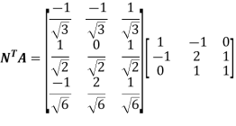
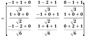
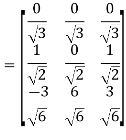
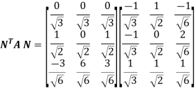
- Find

- Find D (D =

Example 1: Reduce the following quadratic form to canonical form by orthogonal transformation. Also, find rank, index, signature and nature of quadratic form.

Solution: 
Characteristic eq, of matrix A is


For  , Eigen Vector,
For  , Eigen Vector,
For  , Eigen Vector,
Length of eigen vector, 
Length of eigen vector, 
Length of eigen vector, 
Normalised eigen vectors are:
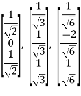
Modal matrix P (Normalised Eigen vector as its column vectors)
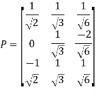
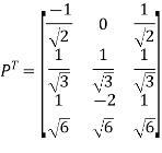
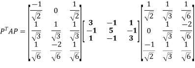

Hence, the canonical form is


Rank (r) = 3 (No. Of non-zero eigen values)
Index = 3 (no. Of positive eigen values)
Example 2: Reduce the quadratic form  to the canonical form through an orthogonal transformation.
Solution: 

To find the characteristic equation.,


 = 0 ,
= 0 , 
To find the eigenvectors,
Case-1,
If 
(A- )X=0
)X=0


Case(2),
If 
(A- )X = 0.


From equation ….(1)
Put  in equation …(2)


Case (3),
If 
(A- )X = 0


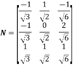
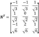
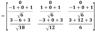
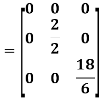
D = 

Textbooks:
1. Erwin Kreyszig, Advanced Engineering Mathematics, 10/e, John Wiley & Sons, 2011.
2. B. S. Grewal, Higher Engineering Mathematics, 44/e, Khanna Publishers, 2017.
References:
1. R. K. Jain and S. R. K. Iyengar, Advanced Engineering Mathematics, 3/e, Alpha Science
International Ltd., 2002.
2. George B. Thomas, Maurice D. Weir and Joel Hass, Thomas Calculus, 13/e, Pearson
Publishers, 2013.
3. Glyn James, Advanced Modern Engineering Mathematics, 4/e, Pearson publishers, 201.
