Unit -7
Recursion
In programming languages, if a program allows you to call a function inside the same function, then it is called a recursive call of the function.
void recursion() {
recursion(); /* function calls itself */
}
int main() {
recursion();
}
The C programming language supports recursion, i.e., a function to call itself. But while using recursion, programmers has to be careful to define an exit condition from the function, otherwise it will go into an infinite loop.
Recursive functions are useful to solve many mathematical problems, such as calculating the factorial of a number, generating Fibonacci series, etc.
The following example calculates the factorial of a given number using a recursive function −
#include <stdio.h>
unsigned long long int factorial(unsigned int i) {
if(i <= 1) {
return 1;
}
return i * factorial(i - 1);
}
int main() {
int i = 12;
printf("Factorial of %d is %d\n", i, factorial(i));
return 0;
}
When the above code is compiled and executed, it produces the following result −
Factorial of 12 is 479001600
The following example generates the Fibonacci series for a given number using a recursive function −
#include <stdio.h>
int fibonacci(int i) {
if(i == 0) {
return 0;
}
if(i == 1) {
return 1;
}
return fibonacci(i-1) + fibonacci(i-2);
}
int main() {
int i;
for (i = 0; i < 10; i++) {
printf("%d\t\n", fibonacci(i));
}
return 0;
}
When the above code is compiled and executed, it produces the following result −
0
1
1
2
3
5
8
13
21
34
Recursion is a common form of the general-purpose problem-solving technique called divide and conquer''. The principle of divide-and-conquer, is that you solve a given problem P in 3 steps:
- divide P into several subproblems, P1,P2,...Pn.
- solve, however you can, each of the subproblems to get solutions S1...Sn.
- Use S1...Sn to construct a solution to the original problem, P.
This is often recursive, because in order to solve one or more of the subproblems, you might use this very same strategy. For instance, you might solve P1 be subdividing it into P1a,P1b..., solving each one of them, and putting together their solutions to get the solution S1 to problem P1.
Suppose we wished to sort the values in array X between positions FIRST and LAST. We can solve this directly in two very simple cases:
FIRST=LAST:
there is one number to be sorted, nothing needs to be done.
FIRST+1=LAST:
there are 2 numbers to be sorted; compare them and, if they are out of order, swap them.
Otherwise, there are too many numbers to be sorted all at once, so we divide the problem into two subproblems by dividing the array into two parts:
- P1: sort the numbers in X between positions FIRST and M; the answer is S1.
- P2: sort the numbers in X between positions M+1 and LAST; the answer is S2.
The final answer is obtained by combining S1 and S2 in an appropriate way. The method for combining them is called merging', and it is a simple, efficient process.
The exact way we divide up the array does not affect the correctness of this strategy: M can be any value at all, FIRST<M<LAST. Certain values of M correspond to well-known sorting algorithms:
M = 1
gives rise to the sorting algorithm called insertion sort.
M = the midpoint between FIRST and LAST
gives rise to the MergeSort algorithm.
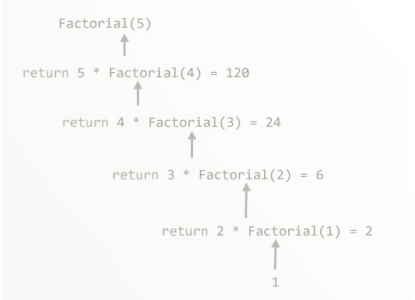
The factorial of a positive number is the product of the integral values from 1 to number itself.
Eg. 5!=5*4*3*2*1
120
Recursive Factorial:

 The factorial algorithm can be defined recursively as follows
Factorial(n) =  1 if n=0
n*(Factorial(n-1)) if n>0
Algorithm:
Calculate factorial of n
fact(n)
- if (n equals 0 )
return 1
2. else
return(n*fact(n-1))
3. endif
end fact(n)
|
Fig.9 Recursive Factorial
P12: Program to find factorial of a number using recursion.
#include<stdio.h>
#include<conio.h>
int rec (int x);
void main()
{
int a, fact;
printf("\nEnter any number: ");
scanf ("%d", &a);
fact=rec(a);
printf("\nFactorial Value = %d", fact);
getch();
}
int rec (int x)
{
int f;
if (x==1)
return (1);
else
f=x*rec(x-1);
return (f);
}
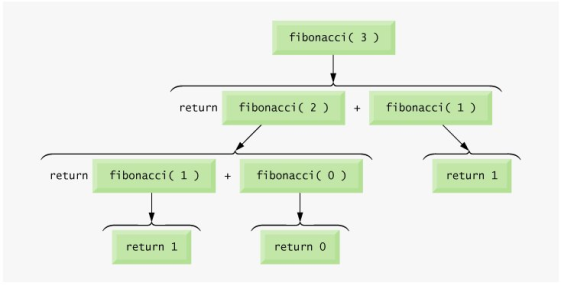
The first two numbers of Fibonacci series are 0,1. The next number is the sum of previous two numbers.
Eg. 0, 1, 1, 2, 3, 5, 8, 13, 21, 34, ...
- 1 is calculated by adding previous two numbers(0+1)
- 2 is calculated by adding the two numbers before it (1+1)
- Similarly, the 3 is found by adding the two numbers before it (1+2), and so on.
FIBONACCI SERIES using RECURSION:


Fibonacci(n) =  0 if n=0
1 if n=1
Fibonacci(n-1)+Fibonacci(n-2)) otherwise
Algorithm:
int fib(int n)
{
- if (n <= 1)
return n;
2. else
return (fib(n-1) + fib(n-2));
}
|
Fig.10 Fibonacci series using Recursion
P13: Program to print Fibonacci series using recursion.
#include<stdio.h>
#include<conio.h>
int Fibonacci(int);
void main()
{
int n, i, c=0;// n is no. of terms in Fibonacci series.
printf(“Enter no. of terms in Fibonacci series”);
scanf("%d",&n);
printf("Fibonacci series\n");
for( i= 1 ; i <= n ; i++ )
{
printf("%d\n", Fibonacci(c));
c++;
}
getch();
}
int Fibonacci(int x)
{
if ( x == 0 )
return 0;
else if ( x == 1 )
return 1;
else
return ( Fibonacci(x-1) + Fibonacci(x-2) );
}
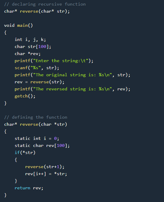
Recursive function (reverse) takes string pointer (str) as input and calls itself with next location to passed pointer (str+1). Recursion continues this way, when pointer reaches ‘\0’, all functions accumulated in stack print char at passed location (str) and return one by one.
|
#include<stdio.h>
#include<conio.h>
int rec (int x);
void main()
{
int a, fact;
printf("\nEnter any number: ");
scanf ("%d", &a);
fact=rec(a);
printf("\nFactorial Value = %d", fact);
getch();
}
int rec (int x)
{
int f;
if (x==1)
return (1);
else
f=x*rec(x-1);
return (f);
}
Merge Sort
Merge Sort is based on divide and conquer strategy. It divides the unsorted list into n sublists such that each sublist contains one element. Each sublist is then sorted and merged until there is only one sublist.
Step 1 : Divide the list into sublists such that each sublist contains only one element.
Step 2 : Sort each sublist and Merge them.
Step 3 : Repeat Step 2 till the entire list is sorted.
Example : Apply Merge Sort on array A= {85,24,63,45,17,31,96,50}
Step1 : A contains 8 elements. First we divide the list into two sublists such that each sublist contains 4 elements. Then we divide each sublist of 4 elements into sublist of two elements each. Finally every sublist contains only one element.
|
Fig. 4.4
Step 2 : Now we start from bottom. Compare 1st and 2nd element. Sort and merge them. Apply this for all bottom elements.
Thus we got 4 sublists as follows
24 | 85 |
| 45 | 63 |
| 17 | 31 |
| 50 | 96 |
Step 3 : Repeat this sorting and merging until entire list is sorted. Thus above four sublists are sorted and merged to form 2 sublists.
24 | 85 | 63 | 85 |
| 17 | 31 | 50 | 96 |
Finally above 2 sublists are again sorted and merged in one sublist.
17 | 24 | 31 | 45 | 50 | 63 | 85 | 96 |
We will see one more example on merge sort.
Example : Apply merge Sort on array A={10,5,7,6,1,4,8,3,2,9,12,11}
Step 1 :
|
Fig. 4.5
Algorithm for Merge Sort:
Let x = no. of elements in array A
y = no. of elements in array B
C = sorted array with no. of elements n
n = x+y
Following algorithm merges a sorted x element array A and sorted y element array B into a sorted array C, with n = x + y elements. We must always keep track of the locations of the smallest element of A and the smallest element of B which have not yet been placed in C. Let LA and LB denote these locations, respectively. Also, let LC denote the location in C to be filled. Thus, initially, we set
LA : = 1,
LB : = 1 and
LC : = 1.
At each step , we compare A[LA] and B[LB] and assign the smaller element to C[LC].
Then
LC:= LC + 1,
LA: = LA + 1, if new element has come from A .
LB: = LB + 1, if new element has come from B.
Furthermore, if LA> x, then the remaining elements of B are assigned to C;
 LB >y, then the remaining elements of A are assigned to C.
Thus the algorithm becomes
MERGING ( A, x, B, y, C)
1. [Initialize ] Set LA : = 1 , LB := 1 AND LC : = 1
2. [Compare] Repeat while LA <= x and LB <= y
If A[LA] < B[LB] , then
(a) [Assign element from A to C ] set C[LC] = A[LA]
(b) [Update pointers ] Set LC := LC +1 and LA = LA+1
Else
(a) [Assign element from B to C] Set C[LC] = B[LB]
(b) [Update Pointers] Set LC := LC +1 and LB = LB +1
[End of loop]
3. [Assign remaining elements to C]
If LA > x , then
Repeat for K= 0 ,1,2,........,y–LB
Set C[LC+K] = B[LB+K]
[End of loop]
Else
Repeat for K = 0,1,2,......,x–LA
Set C[LC+K] = A[LA+K]
[End of loop]
4. Exit
Program for Merge Sort
#include<stdio.h>
#define MAX 50
void mergeSort(int A[],int first,int mid,int high);
void divide(int A[],int first,int last);
int main(){
int merge[MAX],i,n;
printf("Enter the total number of elements: ");
scanf("%d",&n);
printf("Enter the elements which to be sort: ");
for(i=0;i<n;i++){
scanf("%d",&merge[i]);
}
divide(merge,0,n–1);
printf("After merge sorting elements are: ");
for(i=0;i<n;i++){
printf("%d ",merge[i]);
}
return 0;
}
void divide(int A[],int first, int last)
{
int mid;
if(first<last){
mid=(first+last)/2;
divide(A,first,mid);
divide(A,mid+1,last);
mergeSort(A,first,mid,last);
}
}
void mergeSort(int A[],int first,int mid,int last)
{
int i,m,k,l,temp[MAX];
l=first;
i=first;
m=mid+1;
while((l<=mid)&&(m<=last)){
if(A[l]<=A[m]){
temp[i]=A[l];
l++;
}
else{
temp[i]=A[m];
m++;
}
i++;
}
if(l>mid){
for(k=m;k<=last;k++){
temp[i]=arr[k];
i++;
}
}
else{
for(k=l;k<=mid;k++){
temp[i]=arr[k];
i++;
}
}
for(k=first;k<=last;k++){
A[k]=temp[k];
}
}
Output :
Enter the total number of elements: 5
Enter the elements which to be sort: 3 1 6 4 7
After merge sorting elements are: 1 3 4 6 7
Complexity of Merge Sort :
Time to merge two arrays each N/2 elements is linear, i.e. N
Thus we have:
(1) T(1) = 1
(2) T(N) = 2T(N/2) + N
Dividing (2) by N we get:
(3) T(N) / N = T(N/2) / (N/2) + 1
N is a power of two, so we can write
(4) T(N/2) / (N/2) = T(N/4) / (N/4) +1
(5) T(N/4) / (N/4) = T(N/8) / (N/8) +1
(6) T(N/8) / (N/8) = T(N/16) / (N/16) +1
(7) ……
(8) T(2) / 2 = T(1) / 1 + 1
Adding equations (3) through (8), the sum of their left–hand sides will be equal to the sum of their right–hand sides:
T(N) / N + T(N/2) / (N/2) + T(N/4) / (N/4) + … + T(2)/2
= T(N/2) / (N/2) + T(N/4) / (N/4) + ….+ T(2) / 2 + T(1) / 1 + LogN
(LogN is the sum of 1s in the right–hand sides)
After crossing the equal term, we get
(9) T(N)/N = T(1)/1 + LogN
T(1) is 1, hence we obtain
(10) T(N) = N + NlogN = O(NlogN)
Hence the complexity of the MergeSort algorithm is O(NlogN).
Quick Sort
Quick sort is most efficient method of sorting .It uses divide and conquer strategy to sort the elements. In quicksort, we divide the array of items to be sorted into two partitions and then call the quicksort procedure recursively to sort the two partitions. For this we choose a pivot element and arrange all elements such that all the elements in the left part are less than the pivot and all those in the right part are greater than it.
Algorithm to implement Quick Sort is as follows.
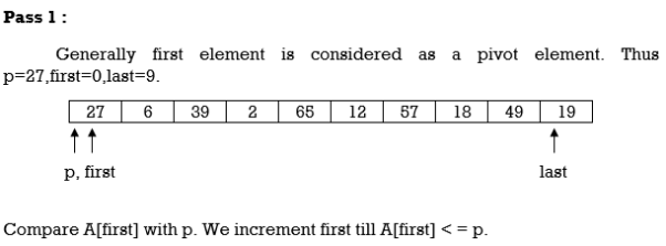
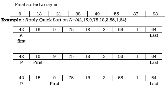
Consider array A of size n to be sorted. p is pivot element. Index positions of first and last element of array A is denoted by ‘first’ and ‘last’.
- Intially first=0 and last=n–1.
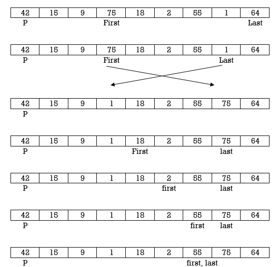
- Increment first till A[first]<=p
- Decrement last till A[last]>=p
- If first < last then swap A[first] with A[last].
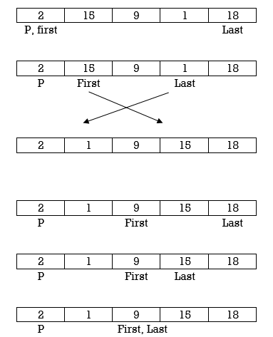
- If first > last then swap p with A[last] and thus position of p is found. Pivot p is placed such that all elements to its left are less than it and all elements right to it are greater than it. Let us assume that j is final position of p. Then A[0] to A[j–1] are less than p and A [j + 1] to A [n–1]are greater than p.
- Now we consider left part of array A i.e A[0] to A[j–1].Repeat step 1,2,3 and 4. Apply same procedure for right part of array.
- We continue with above steps till no more partitions can be made for every subarray.
C function for Quick sort
x=0,y=n–1
void Quicksort(A,x,y)
{
if(x<y)
{
first=x;
last=y;
p=A[x];
while(first<last)
{
while(A[first]<p)
first++;
while(A[last]>p)
last ––;
if(first<last)
swap(A[first],A[last])
}
swap(A[x],A[y])
Quicksort(A,x,last–1);
Quicksort(A,first+1,y);
}
We will see examples on Quick sort
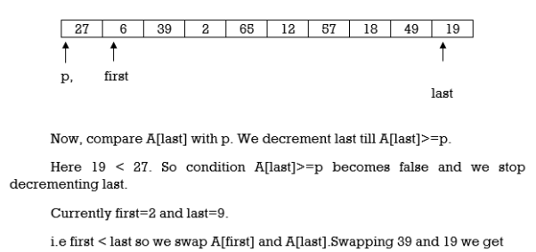
Example : Apply Quicksort on array
A= {27,6,39,2,65,12,57,18,49,19}
|
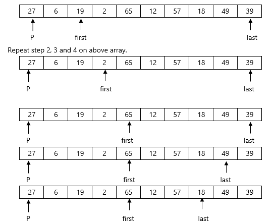
|
Here again first<last so we swap A[first] and A[last]. Swapping 65 and 18 we get
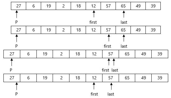
Repeat step 2,3 and 4.
|
Now First>last so we swap pivot p with A[last]. Swapping 27 and 12 we get
12 | 6 | 19 | 2 | 18 | 27 | 57 | 65 | 49 | 39 |
Here we complete Pass 1.Now pivot element is 27 and it divides array in left and right partition. We can see that elements less than pivot are in left partition and elements greater than pivot are in right partition.
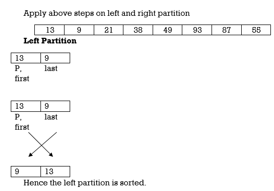
Now we continue same procedure for left and right partition. Here we see results of corresponding passes.
Pass 2 :
12 | 6 | 19 | 2 | 18 | 27 | 57 | 65 | 49 | 39 |
Pass 3 :
2 | 6 | 12 | 19 | 18 | 27 | 57 | 65 | 49 | 39 |
Pass 4 :
2 | 6 | 12 | 18 | 19 | 27 | 57 | 65 | 49 | 39 |
Pass 5 :
2 | 6 | 12 | 18 | 19 | 27 | 49 | 39 | 57 | 65 |
Pass 6 :
2 | 6 | 12 | 18 | 19 | 27 | 39 | 49 | 57 | 65 |
Pass 7 :
2 | 6 | 12 | 18 | 19 | 27 | 39 | 49 | 57 | 65 |
We will see another example.
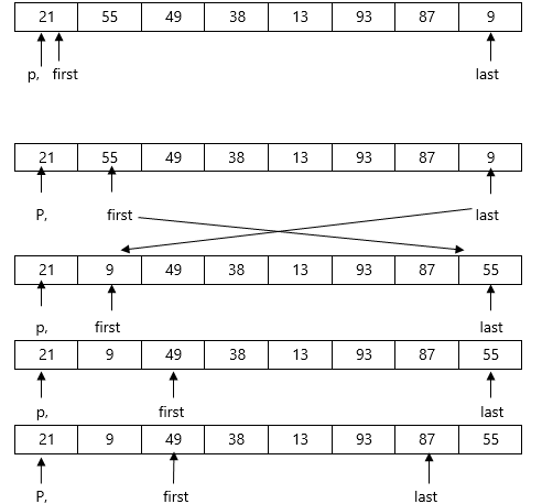
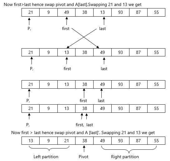
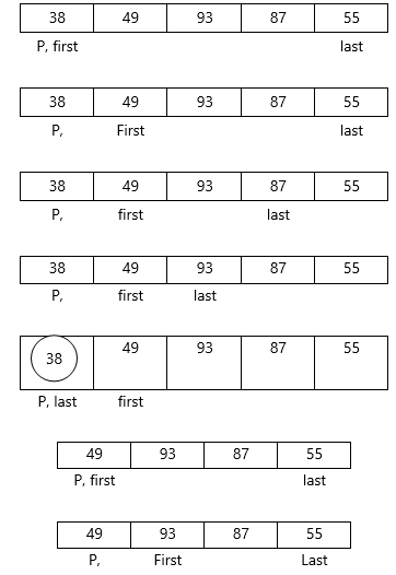
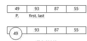
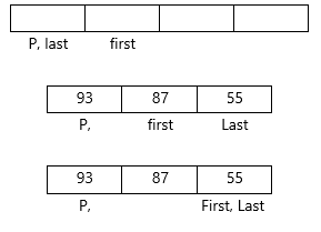
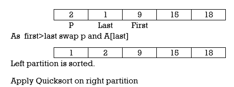
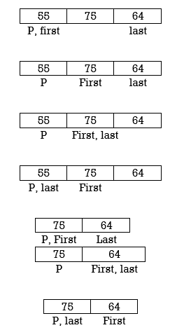
Example : Apply Quicksort on array A={21,55,49,38,13,93,87,9}
Pass 1 :
|
|
|
Considering right partition
|
|
|
|
Hence the right partition is sorted .
|
Swap p and A[last]
|
Applying
|
Program for Quick Sort:
#include<stdio.h>
void quicksort(int A[10],int,int);
int main(){
int A[20],n,i;
printf("Enter size of the array: ");
scanf("%d",&n);
printf("Enter %d elements: ",n);
for(i=0;i<n;i++)
scanf("%d",&A[i]);
quicksort(A,0,n–1);
printf("Sorted elements: ");
for(i=0;i<n;i++)
printf(" %d",A[i]);
return 0;
}
void quicksort(int A[20],int first, int last)
{
int pivot,j,temp,i;
if(first<last){
pivot=first;
i=first;
j=last;
while(i<j){
while(A[i]<=A[pivot]&&i<last)
i++;
while(A[j]>A[pivot])
j––;
if(i<j){
temp=A[i];
A[i]=A[j];
A[j]=temp;
}
}
temp=A[pivot];
A[pivot]=A[j];
A[j]=temp;
quicksort(A,first,j–1);
quicksort(A,j+1,last);
}
}
Output :
Enter size of the array: 5
Enter 5 elements: 3 8 0 1 2
Sorted elements: 0 1 2 3 8
Complexity of Quick Sort
The time to sort the file is equal to
- the time to sort the left partition with i elements, plus
- the time to sort the right partition with N–i–1 elements, plus
- the time to build the partitions
Worst case analysis
The pivot is the smallest element
T(N) = T(N – 1) + cN, N > 1
T(N – 1) = T(N – 2) + c(N – 1)
T(N – 2) = T(N – 3) + c(N – 2)
T(N – 3) = T(N – 4) + c(N– 3)
T(2) = T(1) + c.2
Add all equations:
T(N) + T(N – 1) + T(N – 2) + … + T(2) =
= T(N – 1) + T(N – 2) + … + T(2) + T(1) + c(N) + c(N – 1) + c(N – 2) + … + c.2 |
T(N) = T(1) + c times (the sum of 2 thru N)
= T(1) + c(N(N+1)/2 –1) = O(N2)
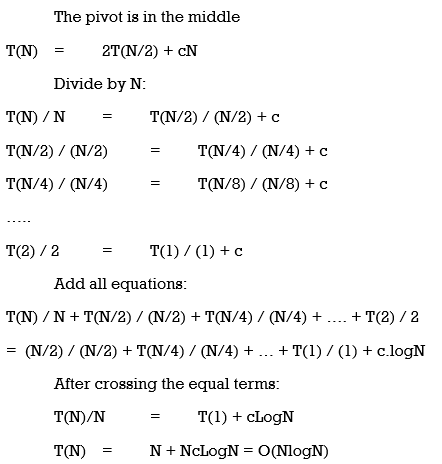
Best–case analysis:
Average case analysis Similar computations, resulting in T(N) = O(NlogN) The average value of T(i) is 1/N times the sum of T(0) through T(N–1) 1/N S T(j), j = 0 thru N–1 T(N) = 2/N (S T(j)) + cN Multiply by N NT(N) = 2(S T(j)) + cN*N To remove the summation, we rewrite the equation for N–1: (N–1)T(N–1) = 2(S T(j)) + c(N–1)2, j = 0 thru N–2 and subtract: NT(N) – (N–1)T(N–1) = 2T(N–1) + 2cN –c NT(N) = (N+1)T(N–1) + 2cN Divide by N(N+1): T(N)/(N+1) = T(N–1)/N + 2c/(N+1) T(N)/(N+1) = T(N–1)/N + 2c/(N+1) T(N–1)/(N) = T(N–2)/(N–1)+ 2c/(N) T(N–2)/(N–1) = T(N–3)/(N–2) + 2c/(N–1) …. T(2)/3 = T(1)/2 + 2c /3 Add the equations and cross equal terms: T(N)/(N+1) = T(1)/2 +2c S (1/j), j = 3 to N+1 The sum S (1/j), j =3 to N–1, is about LogN Thus T(N) = O(NlogN)
|
Reference
- Brian W. Kernighan And Dennis M. Ritchie, The C Programming Language, Prentice Hall Of India
- Yashwant Kanetkar, Let Us C, Bpb Publication
