UNIT 1

Introduction To Control Problem

1.1   Introduction

Definition of control system: A control system is an arrangement of physical components connected or related in such a manner as to command, direct, or regulate itself or another system, or is that means by which any quantity of interest in a system is maintained or altered in accordance with a desired manner.

1.2 Industrial control examples

Control systems are indispensable in modern industrial processes. We find control systems in all sectors of industry, such as quality control of manufactured products, automatic assembly line, machine-tool control, space technology and weapon systems, transportation systems, power systems, robotics, and many others.

a) Automobile driving system

The system to be controlled has two inputs (steering, and acceleration/braking) and two controlled outputs (heading, and speed). The two command inputs are the direction of the highway, and speed limits with traffic signals. A block diagram of this two-input, two-output system is shown in Figure.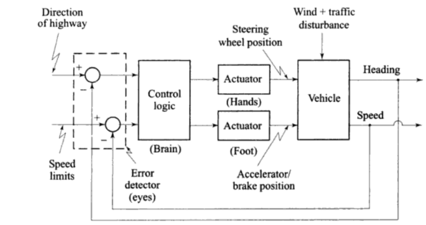

b) Hydraulic Power Steering Mechanism

Many automobiles have power steering which utilizes hydraulic amplifiers for the amplification of the force applied to the wheels. A schematic diagram of the hydraulic power steering mechanism is shown in Figure 2 below. The command input to the system is the rotation of the steering wheel by the driver and the controlled output is the vehicle heading, in a command-following mode (note that the hydraulic power steering mechanism is a sub-system of the automobile driving system shown in Figure above).

c) Residential Heating System

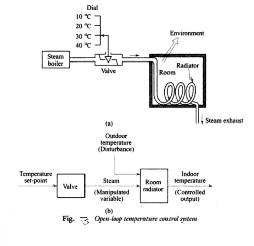
In this system, the indoor temperature is the response variable of interest, and it is affected by the main disturbance input—the outdoor temperature. In the scheme of figure 3 shown below, the desired temperature, which is the command-input temperature, is set on a calibrated dial. This positions the valve that admits the steam for circulation through the radiator. The valve dial is calibrated when the environment temperature has certain value. When this value changes significantly, the controlled temperature will deviate from the desired value by a large error and hence precise control will not be realized. The open-loop scheme of figure is used when performance requirements for heating of a residential building are not very stringent.

1.3 Mathematical Modelling of physical system

There are various types of physical systems, namely we have:

1. Mechanical systems
2. Electrical systems
3. Electronic systems
4. Thermal systems
5. Hydraulic systems
6. Chemical systems

Mathematical modelling of a control system is the process of drawing the block diagrams for these types of systems in order to determine their performance and transfer functions.

Here we discuss mathematical modelling of electrical system.

In an electrical type of system, we have three variables –

1. Voltage which is represented by ‘V’.
2. Current which is represented by ‘I’.
3. Charge which is represented by ‘Q’.

And also, we have three parameters which are active and passive components:

1. Resistance which is represented by ‘R’.

2. Capacitance which is represented by ‘C’.

3. Inductance which is represented by ‘L’.

Now we are in condition to derive analogy between electrical systems.

The following mathematical models are mostly used.

• Differential equation model
• Transfer function model
• State space model

1. Differential Equation Model

Differential equation model is a time domain mathematical model of control systems. Follow these steps for differential equation model.

• Apply basic laws to the given control system.
• Get the differential equation in terms of input and output by eliminating the intermediate variable(s).

Example

Consider the following electrical system as shown in the following figure. This circuit consists of resistor, inductor and capacitor. All these electrical elements are connected in series. The input voltage applied to this circuit is vi

And the voltage across the capacitor is the output voltage vo.

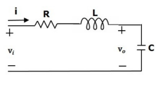
Mesh equation for this circuit is

Substitute, the current passing through capacitor i=c (dv/dt) in the above equation.

The above equation is a second order differential equation.

2. Transfer Function Model

Transfer function model is an s-domain mathematical model of control systems. The Transfer function of a Linear Time Invariant (LTI) system is defined as the ratio of Laplace transform of output and Laplace transform of input by assuming all the initial conditions are zero. If x(t) and y(t) are the input and output of an LTI system, then the corresponding Laplace transforms are X(s) and Y(s). Therefore, the transfer function of LTI system is equal to the ratio of Y(s) and X(s).

The transfer function model of an LTI system is shown in the following figure.

Here, we represented an LTI system with a block having transfer function inside it. And this block has an input X(s)& output Y(s).

Example

Previously, we got the differential equation of an electrical system as

Apply Laplace transform on both sides

Where, vi(s) is the Laplace transform of the input voltage vi and vo(s) is the Laplace transform of the output voltage vo

The above equation is a transfer function of the second order electrical system. The transfer function model of this system is shown below.

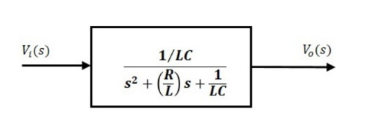
Here, we show a second order electrical system with a block having the transfer function inside it. And this block has an input Vi(s)& an output Vo(s)

1.4 Transfer function models of linear time-invariant systems

We can define the transfer function of a linear time-invariant system as the Laplace transform of the impulse response of the system.

‘The transfer function can also be defined as

Where y(s)=laplace transform of the output variable

R(S)=laplace transform of the input variable r(t) and

G(S)= transfer function of the system

Thus, the transfer function of a time-invariant system is the ratio of the

Laplace transforms of its output and input variables, assuming zero initial

Conditions. Below figure gives a block diagram of a SISO system in transform domain.

Note that whenever a transfer function is used to describe a system, the system is always implicitly assumed to be linear, time-invariant, and relaxed at t0=0.

There are two different ways in which transfer function models ae usually obtained,

(i) For lumped linear time-invariant systems, mathematical model building based on physical laws normally results in a set of (first-order, and second-order) differential equations. Applying Laplace transform to the differential equations result in a transfer function model of the system.

(ii) The transfer function model of a system can be identified from experimentally obtained input-output data. Generally, the identification methods can be considered to be a type of curve-fitting, where the assumed transfer function is fitted to the available data in some optimal manner. The methods may be based on frequency response (sinusoidal input), step response (step input), impulse response (pulse input; pulse of small width approximating an impulse), or the response to more general inputs.

1.5   Feedback Control: Open-Loop and Closed-loop systems

Control Systems can be classified as open loop control systems and closed loop control systems based on the feedback path.

In open loop control systems, output is not fed-back to the input. So, the control action is independent of the desired output.

The following figure shows the block diagram of the open loop control system.

Here, an input is applied to a controller and it produces an actuating signal or controlling signal. This signal is given as an input to a plant or process which is to be controlled. So, the plant produces an output, which is controlled. The traffic lights control system which we discussed earlier is an example of an open loop control system.

In closed loop control systems, output is fed back to the input. So, the control action is dependent on the desired output.

The following figure shows the block diagram of negative feedback closed loop control system.

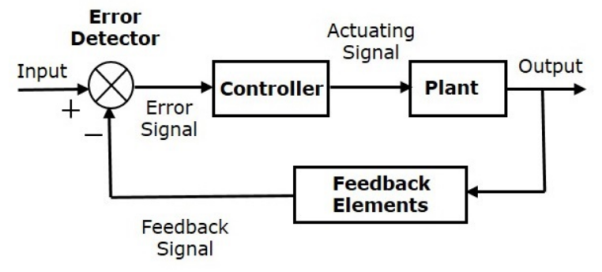
The error detector produces an error signal, which is the difference between the input and the feedback signal. This feedback signal is obtained from the block (feedback elements) by considering the output of the overall system as an input to this block. Instead of the direct input, the error signal is applied as an input to a controller.

So, the controller produces an actuating signal which controls the plant. In this combination, the output of the control system is adjusted automatically till we get the desired response. Hence, the closed loop control systems are also called the automatic control systems. Traffic lights control system having sensor at the input is an example of a closed loop control system.

The differences between the open loop and the closed loop control systems are mentioned in the following table.

1.6  Benefits of feedback

Feedback systems play an important role in control engineering practice because the use of feedback can accomplish certain desirable results that would not be readily possible with an open-loop system. Some of the potential benefits of feedback are explained below.

a) System sensitivity

A process represented by the transfer function G(s), whatever its nature, is subject to modeling errors, changing environment, aging, and other natural factors that affect the control system performance. The use of feedback in reducing sensitivity to parameter variations is an important advantage of the feedback control systems. To have a highly accurate open-loop system, the components of the process plant must be carefully selected so that the parameters of the physical system are close to that of G(s)—the mode! Used in design, under all operating conditions. On the other hand, a closed-loop system allows G(s) to be less accurately specified, since the effects of parameter variations are mitigated by the use of feedback. However, a closed-loop system requires careful selection of the components of the feedback sensor.

b) Disturbance rejection

For accurate rejection of disturbances, the loop gain must be increased in such a manner that the gain from the disturbance input to the system output is not increased.

c) Shaping the dynamic response

With the introduction of feedback system becomes insensitive to model uncertainties.

1.7 Block diagram algebra

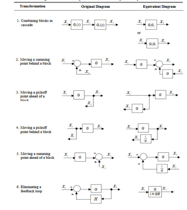
The process by which we can manipulate the block diagrams is nothing more than the manipulation of a set of algebraic transform equations. We can, in fact, manipulate a complex block diagram directly by using the simple rules of block diagram reduction. The most commonly encountered block diagram operations are summarized in table below.

1.8 Signal flow graph

Signal flow graph is a graphical representation of algebraic equations.

Basic Elements of Signal Flow Graph

Nodes and branches are the basic elements of signal flow graph.

Node

Node is a point which represents either a variable or a signal. There are three types of nodes — input node, output node and mixed node.

Input Node − It is a node, which has only outgoing branches. Output Node − It is a node, which has only incoming branches. Mixed Node − It is a node, which has both incoming and outgoing branches.

Example

Let us consider the following signal flow graph to identify these nodes.

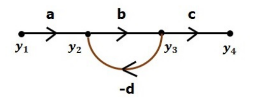
The nodes present in this signal flow graph are y1, y2, y3 and y4. y1 and y4 are the input node and output node respectively. y2 and y3 are mixed nodes.

Branches

Branch is a line segment which joins two nodes. It has both gain and direction. For example, there are four branches in the above signal flow graph. These branches have gains of a, b, c and -d.

Construction of Signal Flow Graph

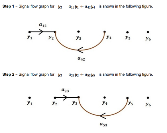
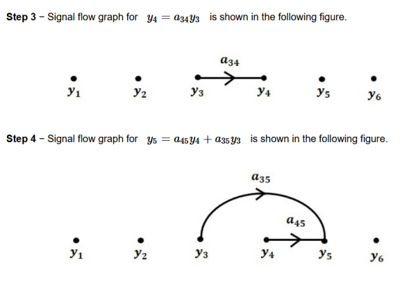
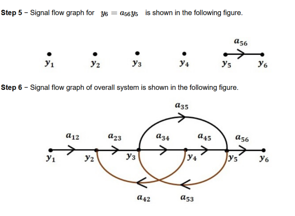
Let us construct a signal flow graph by considering the following algebraic equations –

There will be six nodes (y1, y2, y3, y4, y5 and y6) and eight branches in this signal flow graph. The gains of the branches are a12, a23, a34, a45, a56, a42, a53 and a35.

To get the overall signal flow graph, draw the signal flow graph for each equation, then combine all these signal flow graphs and then follow the steps given below −

Conversion of Block Diagrams into Signal Flow Graphs

Follow these steps for converting a block diagram into its equivalent signal flow graph.

• Represent all the signals, variables, summing points and take-off points of block diagram as nodes in signal flow graph.
• Represent the blocks of block diagram as branches in signal flow graph.
• Represent the transfer functions inside the blocks of block diagram as gains of the branches in signal flow graph.
• Connect the nodes as per the block diagram. If there is connection between two nodes (but there is no block in between), then represent the gain of the branch as one. For example, between summing points, between summing point and take off point, between input and summing point, between take-off point and output.