Unit – 4
Speech Quantization
Figure depicts the input–output characteristics of a uniform quantizer. The quantizer intervals (steps) are all the same duration, as can be seen from its input–output characteristics. The number of quantizer steps and the quantizer step size Δ are the two parameters that describe a uniform quantizer. To allow the most effective use of B bit binary codewords, the number of levels is usually chosen to be of the form 2B. To cover the spectrum of input samples, Δ and B must be chosen together.
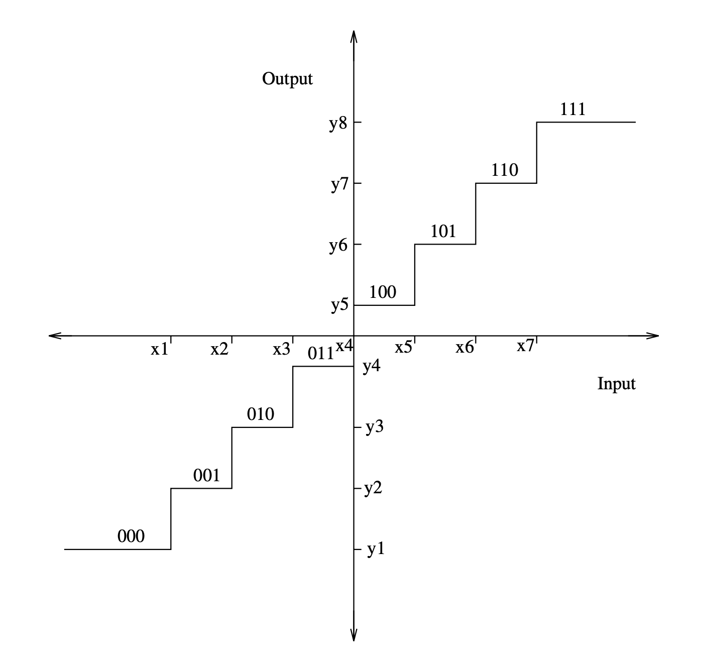
Fig 1: The input–output characteristics of a uniform quantizer
If |x|≤ Xmax and x's probability density function is symmetrical, then
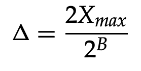
2Xmax = Δ2B
The above equation clearly shows that once the number of bits to be used, B, is defined, the step size Δ can be calculated.
The quantization error eq(n) is bounded by

Increase the number of bits in a uniform quantizer to minimize quantization error. The input signal is presumed to have a uniform probability density function varying between ±Xmax with a constant height of 1/2Xmax . when a uniform quantizer is used.
The input signal's power can be calculated as follows:

The signal-to-noise ratio can be calculated using the following formula:

We get, if we substitute Δ for
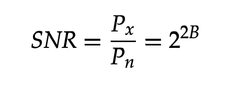
With the log,
SNR(dB) = 10 log10(22B) = 20B log10(2) = 6.02B dB
The above result can be used to estimate the output of a uniform quantizer for a given bit rate as well as to determine the number of bits needed in the quantizer for a given signal to quantization noise ratio.
Key takeaway:
When choosing a quantizer's levels, the placement of these levels must be chosen so that the quantization error is minimized. The levels of the quantizer must be chosen to fit the probability density function of the signal to be quantized in order to optimize the signal to quantization noise ratio for a given number of bits per sample. This is because speech-like signals do not have a uniform probability density function, and smaller amplitudes have a much higher probability of occurring than large amplitudes.
As a result, the best quantizer should have quantization levels of nonuniform spacing to cover the signal dynamic spectrum as accurately as possible. Figure depicts the input–output characteristics of a standard non uniform quantizer, where the quantizer interval phase size increases as the input signal value increases. The probability of the signal dropping through a certain quantization interval determines the noise contribution of each interval. The quantization levels' non uniform spacing is analogous to a nonlinear compressor C(x) followed by a uniform quantizer.
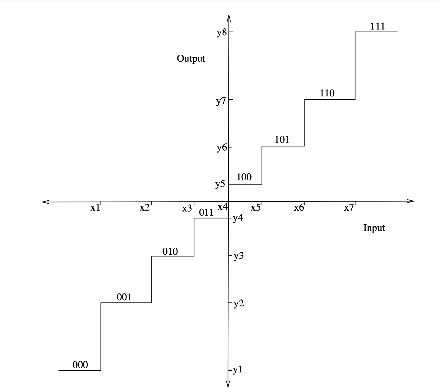
Fig 2: The input–output characteristics of a non-uniform quantizer
C(x) is a nonlinear compressor that compresses input samples based on statistical properties. To put it another way, the lower amplitude samples are compressed rather than the higher amplitude samples. A uniform quantizer is then used to quantize the compressed samples. By applying the inverse C-1(x) expansion to the de-quantized samples at the receiver, the compression effect is reversed. There are no signal distortions as a result of the compression and expansion processes.
Selecting the best compression–expansion combination for a given input signal probability density function is critical. Panter and Dite's study was based on the premise that the quantization was fine enough and that the input samples' amplitude probability density function was constant within the quantization intervals. If the input samples have a peak to root mean squared (rms) ratio greater than 4, their results indicate a substantial improvement in the signal to noise ratio over uniform quantization.
Max [4] discovered how to select the best output levels for nonuniform input quantizer levels when designing an optimum quantizer. His research necessitated prior knowledge of the probability density function as well as the input signal's variance, σx2, but made no assumptions about fine quantization.
For two reasons, nonuniform quantization is useful in speech coding, in both coarse and fine quantization situations. For starters, a non-uniform quantizer suits the speech probability density function better than a uniform quantizer, resulting in a higher signal to noise ratio. Second, a non-uniform quantizer quantizes lower amplitudes more reliably, which contribute more to speech intelligibility.
Key takeaway:
If the dynamic range (or variance) of the input signal is fixed to a small known range, an optimal quantizer is beneficial. However, as the signal's power deviates from the value for which the quantizer was built, the quantizer's output degrades rapidly. While this can be controlled by normalizing the input signal to unit variance, for proper scaling of the de-quantized signal amplitudes, this procedure necessitates the transmission of the signal variance at known time intervals.
Cattermole proposed two companding laws called A-Law and -Law Pulse Code Modulation to account for the broad dynamic range of the input speech signal (PCM). The signal to quantization noise output of both schemes can be very similar to that of a uniform quantizer, but they do not change dramatically with changing signal variance and remain relatively constant over a large range of input speech levels. Companded quantizers need less bits per input sample than uniform quantizers for a given signal dynamic range and signal to quantization noise ratio.
The compression of the A-Law is defined as follows:
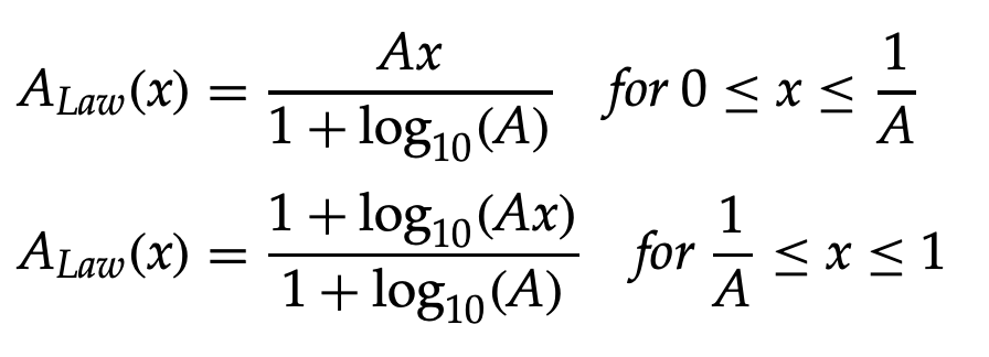
where A is the compression parameter, with standard values of 86 for 7 bit PCM speech quantizers in North America and 87.56 for 8 bit PCM speech quantizers in Europe.
On the other hand, the µ - Law compression is defined as follows:

Where V0 = Lσx is the loading factor and x is the rms value of the input speech signal, and L is the loading factor.
The compression factor is typically set to 255. The A-Law is a combination of a logarithmic curve for large amplitudes and a linear curve for small amplitudes, as shown by the above expressions. In any range, the -Law is not exactly linear or logarithmic, but it is roughly linear for small amplitudes and logarithmic for large amplitudes.
When the channel is idle, an optimal quantizer can have more background noise, and its dynamic range is limited to a narrower input signal range. Logarithmic quantizers are normally chosen for these two purposes.
Key takeaway:
Although the probability density function of speech can be easily measured and used in the quantizer design process, variations in its dynamic range, which can be as much as 30 dB, reduce any quantizer's efficiency. This can be avoided by adjusting the input signal's dynamic range.
As previously mentioned, one way to accomplish this is to estimate the speech segment's variance prior to quantization and then adjust the quantizer levels accordingly. The quantizer levels are adjusted in the same way as the quantizer is designed for unit variance and the input signal is normalized before quantization.
This is referred to as "forward adaptation." If the speech remains stationary for K samples, the rms is calculated as follows:
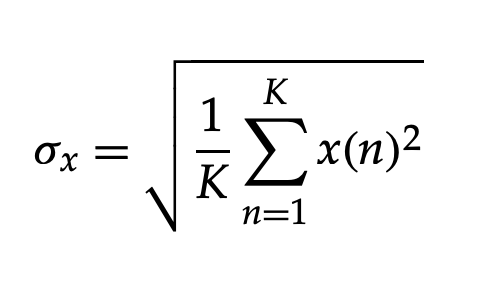
Figure shows a block diagram of a forward adaptive quantizer.
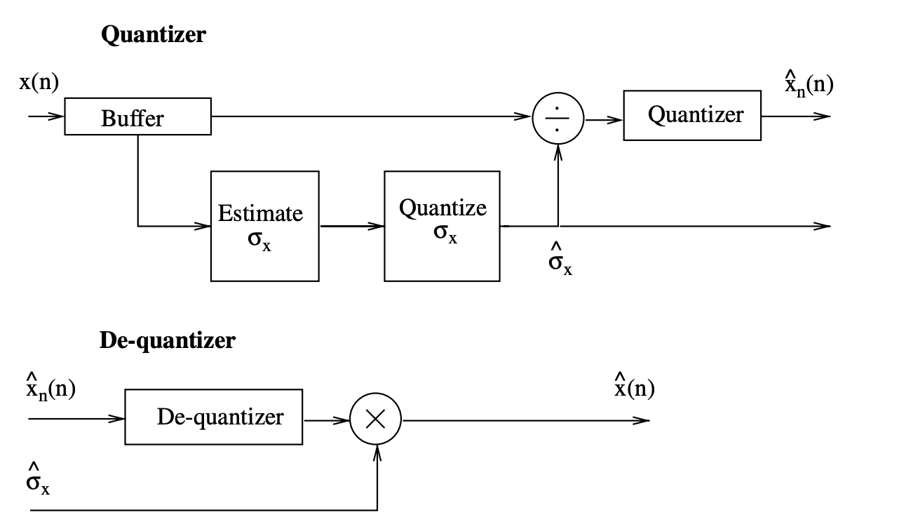
Fig 3: Block diagram of a forward adaptive quantizer
where x(n) represents the speech samples in the block and mean is considered to be zero. The choice of block length K, on the other hand, is critical since K can affect the probability density function of the normalized input signal. The normalized speech signal's probability density shifts from Gaussian (K 128) to Laplacian (K > 512) as K increases.
Both the quantizer and the de-quantizer use a quantized version of the speech rms, σx, to make normalization and denormalization compatible. Backward adaptation is a method of adaptation that does not entail the transmission of speech variation to the de-quantizer. The rms of the input signal is estimated from N previously quantized samples before each sample is quantized. As a result, for the nth sample, the normalizing factor is:
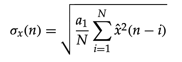
where xˆ denotes the quantized values of previous samples and a1 denotes the tuning factor.
Key takeaway:
The difference between the input samples x(n) and their estimated xp(n)is the difference between the final quantized signal, r(n), in a differential quantizer.
r(n) = x(n) − xp(n)
And
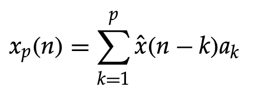
where ak is the weighting applied to the previously quantized (n - k)th sample and p is the number of previously quantized samples taken into account in the calculation.
The explanation for this preprocessing stage to form the prediction residual (prediction error signal) before quantization is that there is a clear correlation between adjacent samples in speech signals, and hence the signal variance is reduced by eliminating some of the redundancies that speech signals have before quantization.
Figures 4 and 5 show block diagrams of typical adaptive differential quantizers.
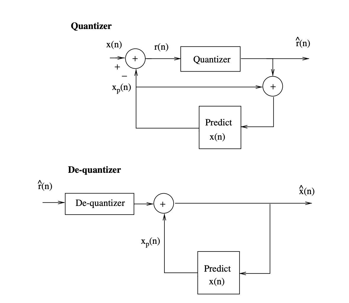
Fig 4: Block diagram of a backward adaptive differential quantizer
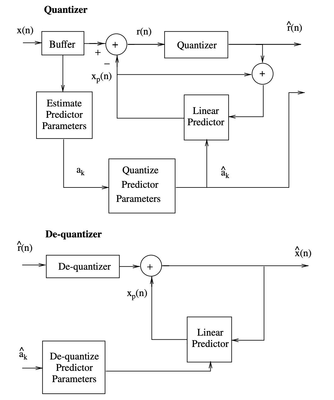
Fig 5: Block diagram of a forward adaptive differential quantizer
Consider the following example to demonstrate the benefits of a differential quantizer over a nondifferential quantizer: Assume that a nondifferential quantizer with a total of K.B1 bits would be used to quantize K input samples. Consider differentially quantizing the same K samples, in which case K error samples ei are quantized to B2 bits/sample accuracy.
The weighting coefficients ak in a differential quantizer can be determined using backward or forward techniques, as shown in Figures 4 and 5. The quantizer does not need to submit extra information to the de-quantizer while using backward estimation of the ak parameters.
In the case of forward estimation of the ak parameters, however, the differential quantizer will also need K.B3 bits to send the ak parameters to the de-quantizer for proper quantized signal recovery. The variance of the error signal to be quantized by the differential quantizer is much smaller than that of the original speech samples since the similarity between the input speech samples is normally strong.
A differential quantizer's output can be roughly characterized by its prediction gain and residual error quantizer's performance.
Key takeaway:
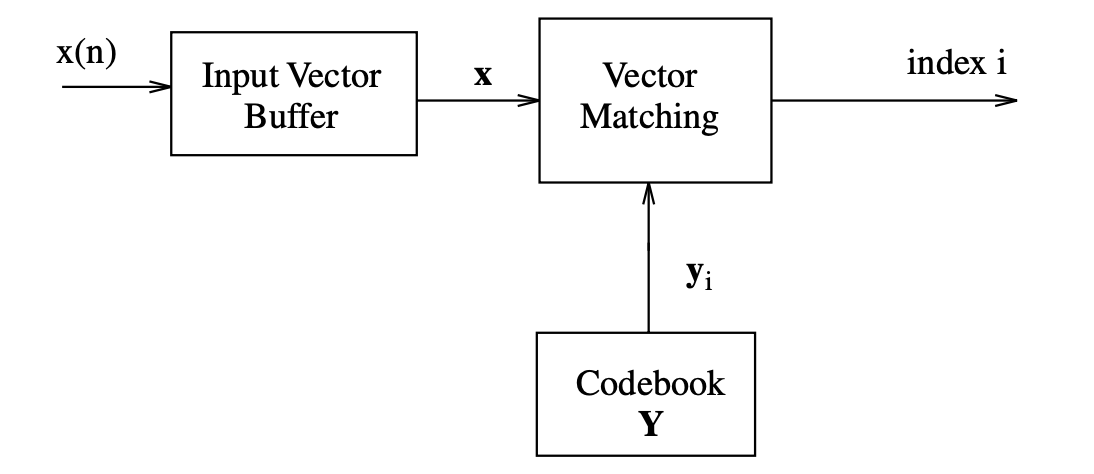
Vector quantization (VQ), also known as block quantization or pattern-matching quantization, is the process of quantizing a group of discrete-time amplitude values as a single vector.
A simple vector quantizer is shown as a block diagram.
Fig 6: Block diagram of a simple vector quantizer
Distortion Measures
A subjectively applicable distortion measure is one in which variations in distortion values may be used to denote equivalent differences in speech content. However, a few decibels of reduction in distortion can be audible in one case but not in another. Although objective distortion tests are important and useful in the design of speech coding systems, subjective quality testing can be used to make decisions on where to improve code efficiency.
Mean Squared Error
The mean squared error (MSE), which is defined as, is the most common distortion measure.

The MSE's success stems from its ease of use.
Weighted Mean Squared Error
The mean squared error method assumes that each part of the vector x contributes an equal amount of distortion. In general, unequal weights may be used to make some elements' contributions to distortion more significant than others. As a result, the general weighted mean squared error is defined as follows:
dw[x, y] = (x − y)W(x − y)T
where W is a weighting matrix with a positive value.
Perceptually Determined Distortion Measures
Reasonable distortion steps, such as the two listed above, work well with similar outputs at high bit rates and thus small distortions.
They also have a good correlation with subjective assessments of speech content.
Simple distortion interventions, on the other hand, may not be related to the subjective quality of speech as the bit rate decreases and distortion increases. Since vector quantization is intended to be used at low bit rates, it's critical to create and use distortion measures that are more closely linked to human auditory behavior.
There have been a number of perceptually dependent distortion measures created. Since the main goal is to achieve the highest possible speech quality at a given bit rate, it's important to use a distortion test that closely resembles human experience.
Key takeaway:
An L level codebook is created by partitioning N dimensional space into L cells Ci, 1 ≤ I ≤ L, and assigning a vector yi to each cell Ci. If x is in Ci, the quantizer selects the codebook variable yi. The distortion in the equation is reduced over all L levels to maximize a quantizer. For optimality to exist, two conditions must be met.
The first condition is that the optimal quantizer minimizes the distortion criterion to find a matching vector for each input vector. That is, the quantizer selects the codebook vector with the least amount of distortion in relation to x.
q(x) = yi if d[x, yi ] ≤ d[ x, yj ], j ≠ i, 1 ≤ j ≤ L.
The second requirement for optimality is that each codebook vector yi is designed to result in the least average distortion in cell Ci.

where p(x) is the probability density function of vectors in cell (cluster) Ci that result in the quantized vector yi.
The centroid of the cell Ci is vector yi. The concept of the distortion measure affects the optimization of a cell's centroid. The distortion in each cell is reduced by, for either the mean squared error or the weighted mean squared error.
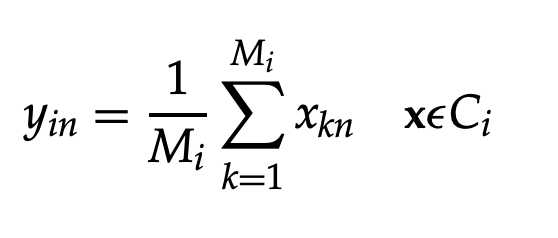
where yin {n = 1, 2,..., N} is the nth member of the cluster Ci's centroid yi. To put it another way, yi is the sample mean of all the training vectors Mi in cell Ci. The K-means algorithm, an iterative clustering algorithm, is one of the most common methods for codebook design.
The algorithm divides the training vectors into L clusters Ci that satisfy the two necessary conditions for optimality.
K-means Algorithm
Given that m is the iteration index, Cim is the ith cluster at iteration m, and yim is the centroid, we may write:
2. Classification: Using the nearest neighbor law, divide the set of training vectors xn, 1 ≤ n ≤ M, into clusters Ci.
x∈Cim if d[x, yim] ≤ d[x, yjm] for all j ≠ i.
3. By computing the centroid of training vectors in each cluster, you can update the codebook vector of each cluster.
4. Stop if the decrease in overall distortion at iteration m relative to iteration 1 is less than a certain threshold; otherwise, proceed to step 2.
For phase 4, some other fair termination test may be used.
The algorithm described above converges to a local optimum. Furthermore, every such solution is not special in general. Global optimality can be approximated by setting the codebook vectors to various values and repeating the above algorithm for multiple sets of initializations before selecting the codebook with the least overall distortion.
Key takeaway:
At very low bit rates, vector quantization will outperform scalar quantization significantly. However, these benefits come at a high cost in terms of computing and energy. A variety of codebook types have been designed to strike a balance between computation and storage costs as well as quantizer efficiency. Some codebooks are pre-computed and do not need to be modified while in use, while others can need to be updated during quantization. We'll go through some of the most commonly used codebooks in speech coding here.
4.8.1 Full Search Codebook
A complete search codebook compares each input vector to all of the candidate vectors in the codebook during the quantization process.
This is referred to as a complete or exhaustive quest. A standard complete search codebook's computing and storage specifications can be estimated as follows. The number of vectors in a complete search codebook is given by, if each vector is represented by B = RN bits for transmission.
L = 2B = 2RN
where N is the codebook's vector dimension. Computing the absolute value of the quantization error might not be appropriate in many applications since the key concern is to choose the best performing vector.
The computation cost (assuming that all the vectors are normalized, as variations in the energy levels would give misleading cross-correlation values) is given by, assuming that the cross-correlation of the input vector with each of the codebook candidates is computed and the one resulting in the highest cross-correlation value is selected as the quantized value of the input vector.
Comfs = N2RN multiply − add per input vector
We can also measure the amount of storage available for the codebook vectors using this formula:
Mfs = NL = N2B = N2RN locations
The computing and storage requirements of a complete search codebook are exponentially proportional to the number of bits in the codewords, as shown by the above expressions.
4.8.2 Binary Search Codebook
Binary search, also known as hierarchical clustering in the pattern recognition literature, is a method of partitioning space in which the search for the least distortion code-vector is proportional to log2 L rather than L. Binary search codebooks are also known as tree codebooks or tree search codebooks in the speech coding literature.
A binary search codebook divides an N-dimensional space into two regions (using the K-means algorithm with two initial vectors), then each of the two regions is further divided into two subregions, and so on, until the space is divided into L regions or cells. L must be a power of two, so L = 2B, where B is an integer number of bits.
A centroid is assigned to each zone. The division of space into L = 8 cells is depicted in the diagram. At the first binary division, the centroids of the two halves of the total area to be filled are determined as v1 and v2. At the second binary division, four centroids, v3 to v6, are determined.
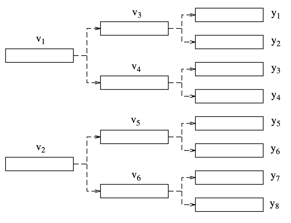
Fig 7: Binary splitting into eight cells
The real codebook vectors yi are the centroids of the regions after the third binary division. The tree is searched along a path that gives the least distortion at each node in the path, using an input vector x. The computation cost would be, assuming N multiply–adds for each distortion computation.
Combs = 2N log2 L = 2NB multiply − add per input vector
The input vector is compared to only two candidates at each point.
4.8.3 Cascaded Codebooks
The main benefit of a binary search codebook is that it has a far lower computational cost than a complete search codebook while sacrificing only a small amount of results. However, as compared to a complete search codebook, the storage needed for a binary search codebook is nearly doubled.
Cascaded vector quantization is a technique for reducing both storage and computational costs. Figure depicts a two-stage cascaded vector quantization. Cascaded vector quantization is made up of a series of vector quantization steps, each of which operates on the previous stage's error signal.
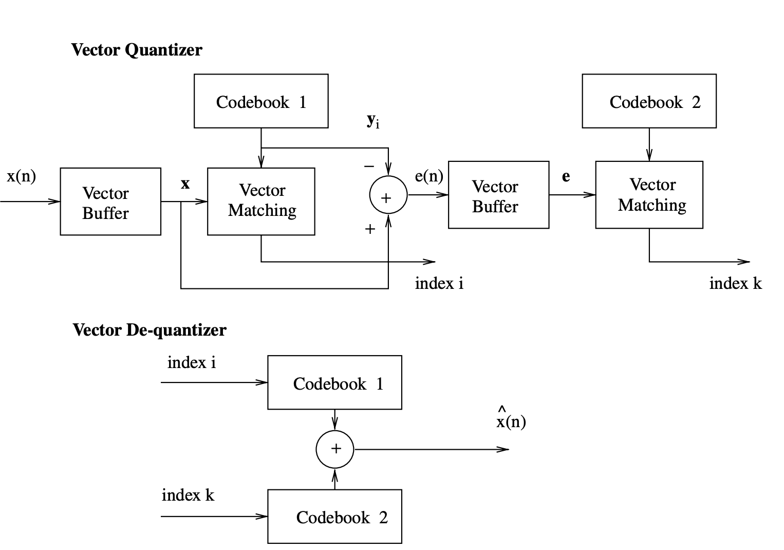
Fig 8: A two-stage cascaded vector quantizer
The input vector x is first quantized with a B1 bit L1 level vector quantizer, and the resulting error signal is then fed into a B2 bit L2 level second vector quantizer as the input. The quantized value of the input vector x is obtained by adding the two quantized vectors.
4.8.4 Adaptive Codebooks
Making a codebook adaptive is one way to make it monitor the input vector characteristics over time. The adaptation of a codebook can be accomplished using either forward or backward schemes, much like an adaptive scalar quantizer.
Before the quantization step, the codebook is modified with respect to the input vectors in a forward adaptive vector quantizer, which necessitates the transmission of certain side information to the de-quantizer for compatible adaptation required for proper signal recovery.
The codebook is modified by the correctly transformed most recent quantizer output vectors in the case of a backward adaptive quantizer. In this case, no side information is needed because the de-quantizer will perform the same update process using the previously recovered vectors.
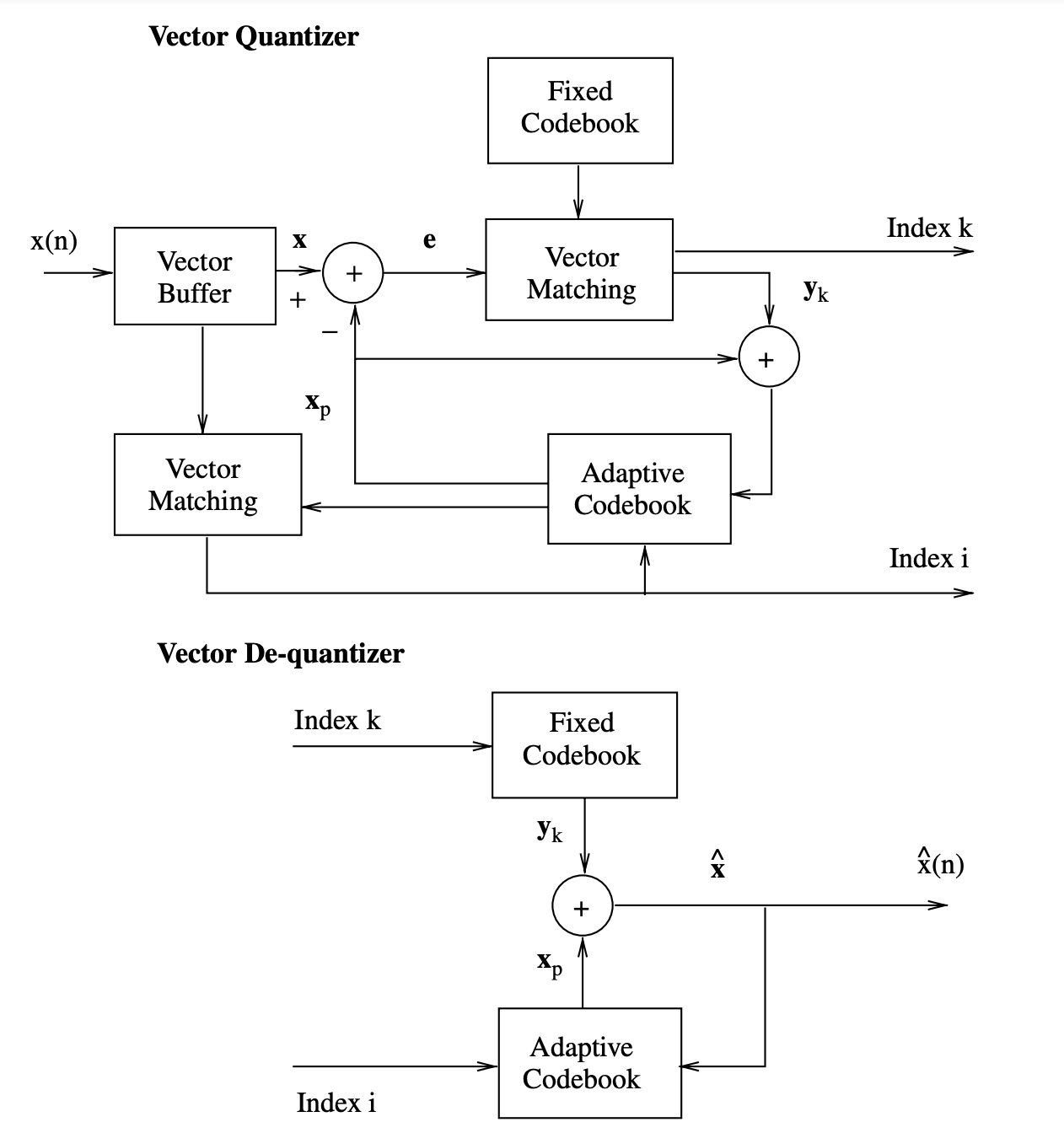
Fig 9: Adaptive vector quantizer in a cascaded setup
An adaptive codebook is typically used in conjunction with other codebooks, which provide the adaptive codebook with initial vectors and aid in the adaptation process when major signal variations occur.
Figure shows an adaptive codebook in a two-stage cascaded vector quantizer. An adaptive codebook can be used in the first stage, followed by a fixed codebook in the second stage. Predictor codebooks are the adaptive codebooks used in these configurations, and the whole process is known as predictive or differential vector quantization.
Key takeaway:
References:
2. “Speech Coding Algorithms: Foundation and Evolution of Standardized Coders”, W.C. Chu, Wiley Inter science, 2003.
