UNIT I

Demand and Supply

1.1           Introduction: Demand and Supply

Demand for goods and services

Economists use the term demand to refer to the amount of some good or service that consumers can happily buy at each price demand is based on needs and wants—consumer’s mite differentiate between desires and wants, but from other point of view demand also pays it on terms of ability. If you cannot pay for it, there is no effective demand.

What the buyer pays for a particular unit of goods or services is called the price. The total number of units purchased at that price is called the requested quantity. An increase in the price of a good or service in most cases reduces the amount of demand for that good or service. On the contrary, the fall in price increases the amount requested. For example, when the price of a gallon of gasoline goes up, people look for ways to reduce consumption by combining several errands, commuting in carpool or mass transit, or taking weekend and vacation trips closer to home. Economists demanded the law of demand, which calls for this inverse relationship between price and volume. The law of demand says that all other changes influencing demand (described in the next module) are kept still

An example from the market of gasoline can be shown in the form of a table or a graph. A table showing the quantity required for each price, as shown in Table 1, is called a demand schedule. The value here is measured in currency as per gallon of gasoline. The amount required is measured in millions of gallons over a period of time (e.g., per day or per year) and over a region (like a state or country). The market curve shows the correlation between price and quantity needed on the graph as shown in Figure 1, with quantity on the horizontal axis and price per gallon on the vertical axis.

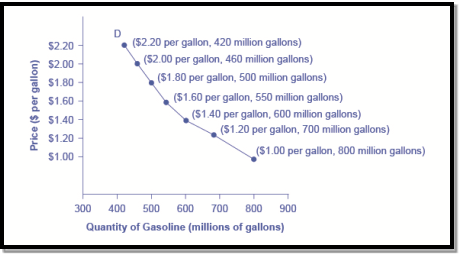
The demand schedule appeared in Table 1 and the demand curve below in the diagram in Figure 1 is two ways to describe the same relationship between price and demand. Figure 1. Demand curve for gasoline. Demand schedule these points are then graphed, and the line connecting them is the demand curve (D). The falling slope of the demand curve shows the demand law —the opposite relationship between the price and the volume of demand. The demand curve appears somewhat different for each product. It is relatively steep or flat that a new straight line or curved surface r. Almost all demand curves share the basic similarity that they are tilted from left to right. Thus, the demand curve expresses the law of demand: as the price increases, the amount requested decreases, and, conversely, as the price decreases, the amount requested decreases.

Is the demand the same as the requested quantity?

In economic terms, demand is not the same as the required quantity. When economists talk about demand, they mean a certain point on the demand curve, or one amount on the demand schedule, as indicated by the demand curve or demand schedule, when economists talk about the range of prices and the quantity requested at those prices and the quantity requested. In short, demand refers to a curve, and demand refers to a (specific) point on the curve.

Supply for goods and services

When economists speak about supply, it means the sum of certain good or service that producers are willing to provide at each price. The worth is what the producer receives for selling one unit of products or services. A rise in cost always tends to a rise within the supply of that goods or service, while a fall in price results in a decrease within the supply. When gasoline prices rise, for instance, it encourages profit—seeking companies to require some action: expand exploration for oil reserves, invest in additional pipelines and oil tankers, and take oil to factories which will refine it into gasoline, build new oil refineries, and switch gasoline into a gasoline station economist. Mist calls this positive relationship between price and supply—that the upper price are going to be the upper supply and therefore the lower cost are going to be the lower supply-the law of supply. The law of supply assumes that each one other variable that affects supply (described within the next module) is kept constant. Still unclear about the various sorts of supply? See the subsequent Clear It Up feature. Is the supply an equivalent because the quantity supplied? In economic terms, supply isn't an equivalent as supply. When economists ask supply, they will be indicated by the availability curve or supply schedule, the connection between the range of costs and therefore the quantity supplied at those prices. When specialist in economics refers to provide, they mention certain point on the availability curve, or one quantity on the availability schedule. In short, supply refers to a curve, and therefore the amount supplied refers to a (specific) point on the curve.

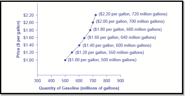
Figure 2 shows the laws of supply, taking the gasoline market as an example. Like demand, supply is often indicated using tables or graphs. The availability graph may be a bit like Table 2, which shows the quantities supplied in several price ranges. Again, the worth is measured in dollars per gallon of gasoline, and therefore the supply is measured in many gallons. The availability curve graphically shows the connection between the worth displayed on the vertical axis and therefore the quantity displayed on the horizontal axis. The availability graph and provide curve are two alternative ways to display equivalent information. Note that the horizontal and vertical axes on the graph of the availability curve are an equivalent as for the demand curve.

Figure 2. Gasoline supply curve. The availability graph may be a table that shows the availability of gasoline at each price. As prices rise, the quantity of supply also increases, and the other way around. A supply curve is made by charting points from a supply graph and connecting them. The upward slope of the availability curve indicates the law of supply—a higher price results in a better supply, and the other way around.

The Shape of the availability curve varies somewhat counting on the product: steep, flat, straight or curved. But most supply curves share a fundamental similarity: they lean left to right and show the law of supply: because the price rises from$1.00 per gallon to$2.20 per gallon, the availability increases from 500 gallons to 720 gallons. On the contrary, because the price decreases, the quantity supplied decreases.

1.2   Determinants of demand

Some of the key determinants of demand are:

【1】Price of the product

When all other factors remain constant or equal, people make decisions with price as a parameter. According to the law of demand, this means that the increase in demand follows the decrease in price, and the decrease in demand follows the increase in the price of similar goods.

The demand curve and demand schedule help you determine the demand quantity at the price level. Elastic demand implies a robust variation with price changes. Similarly, inelastic demand means that even if there is a change in price, the quantity does not change much.

[2] Consumer income

An increase in income leads to an increase in the number of goods demanded by consumers. Similarly, a decrease in income is accompanied by a decrease in the level of consumption. This relationship between income and demand isn't linear in nature. Marginal utility determines the percentage of changes in demand levels.

3] Prices of related goods or services

Complementary products-an increase in the price of one product causes a decrease in the amount required for complementary products. Example: an increase in the price of bread reduces the demand for butter. This occurs because the product is complementary in nature.

Alternative products-an increase in the price of one product causes an increase in demand for alternative products. Example: an increase in the price of tea will increase the demand for coffee and decrease the demand for tea.

4] Consumer expectations

The expectation of higher income or the expectation of an increase in the price of goods leads to an increase in the required amount. Similarly, the expectation of a decrease in income or a decrease in commodity prices would reduce the amount requested.

5] Number of buyers in the market

The number of buyers has a significant impact on aggregate or net demand. As the number increases, the demand increases. In addition, this is true regardless of the change in the price of the goods.

1.3 Movements vs. Shift in demand curve

In the study of economics, it's also important to be ready to distinguish the movement and shift of the demand curve, while understanding the meaning and analysis of the demand curve. During this article, we'll check out the way to understand the difference between moving along the demand curve and shifting the demand curve motion along the demand curve and the demand curve shifting.

Every company faces a particular demand curve for the products it supplies. There are many factors that affect demand, and these effects are often seen by observing changes within the demand curve. Broadly, factors are often weakened into two types:

Demand curve movement

When there's a change within the amount required for a specific commodity, due to the change in price, there's a movement of the quantity required along an equivalent curve, with other factors remaining constant.

An important aspect to recollect is other factors like consumer income and taste alongside other goods like price. It remains constant and only the worth of the products changes.

In such a scenario, the worth change affects the requested quantity, but the demand follows an equivalent curve as before the worth change. This is often the movement of the demand curve. This movement can occur in an upward or downward direction along the demand curve.

We know that if all other factors remain constant, the rise within the price of products will reduce its demand. Also, the drop by prices increases demand. So what happens to the demand curve?

Change in demand

It shows a change within the amount obtained within the figure. 1. The above shows that when the worth of the products is OP, its demand is OM (if other factors are constant). Now, let's check out the impact of the rise and reduce in prices on demand:

When the worth rises from OP to OP, the quantity requested falls to OL. Also, the demand curve moves upwards.

When the worth decreases from OP to OP', the requested amount rises to ON. Also, the demand curve moves downward.

So we will see that price changes, where other factors remain constant, move the demand curve up and down.

Shifting demand curves

The demand curve shifts when there's a change within the required amount of a specific commodity at each possible price thanks to a change in one or more other factors. A crucial aspect to recollect is other factors like consumer income and taste alongside other goods like price. It had been expected to stay constant and altered.

In such a scenario, a change in price, alongside a change in one or more other factors, affects the quantity requested. Therefore, demand follows a special curve for every change in price.

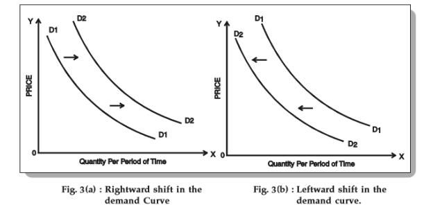
This is the shift within the demand curve. The demand curve can shift to either the left or the proper, counting on the factors affecting it.

Let's check out an example that captures the effect of changes in consumer income on the quantity required.

The demanded quantities are plotted as demand curves DD and D’D’ as shown below:

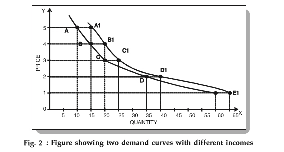From the above figure 2, we can clearly see that as income changes, price changes shift the demand curve. In this case, the shift is on the right, indicating an increased desire to buy goods at all prices.

Thus, it can be concluded that the demand curve shifts to the right with an increase in income. On the other hand, when income declines, the demand curve shifts to the left, which reduces the desire to buy goods.

1.4 Determinants of Supply

While price is an important aspect to determine the willingness and desire to part with a product/service, many other factors determine the supply of a product or service, as described below.

1. Price of goods / services

The most obvious determinant of supply is the price of the product/service. If all other parameters are equal, the higher the relative price will increase the supply of the product. The reason is simple. Companies offer goods and services to make a profit, and when the price goes up, so does the profit.

2.     Related products prices

Let's say the price of wheat has gone up. Therefore, it will be more profitable for the enterprise to supply wheat, compared to corn and soybeans. Thus, the supply of wheat increases, but the supply of corn and soybeans decreases.

Therefore, we can say that if the price of related goods increases, the enterprise will increase the supply of goods with higher prices. This leads to a decrease in the supply of goods with lower prices.

3.     Price of production factors

The production of goods costs a lot. If the price of a particular factor of production increases, the cost of manufacturing goods that use the element in large quantities increases significantly. The cost of production of goods that use the above elements in a relatively small amount increases slightly.

For example, the increase in the cost of land has a significant impact on the cost of wheat production, and a small impact on the cost of production of cars.

So, when the price of one factor of production changes, the relative profitability of different production lines changes. This causes producers to shift from one line to another, resulting in changes in the supply of goods.

4.     Current status of technology

Technological innovations and inventions tend to make it possible to use the same resources to produce better quality and/or quantity of goods. Thus, the state of technology can increase or decrease the supply of certain goods.

5.     Government policy

Goods taxes, such as excise duty, import duty, GST, etc., have a big impact on the cost of production. These taxes could raise the overall cost. Therefore, the supply of goods affected by these taxes will only increase if the price increases. Subsidies, on the other hand, reduce the cost of production, which usually leads to an increase in supply.

6.     Other factors

There are many other factors that affect the supply of goods or services: government industrial and foreign policy, corporate goals, infrastructure facilities, market structure, natural factors.

1.5 Movement along a supply curve vs. Shift in supply curve

Supply curve

The supply curve is the trajectory of all points indicating the different quantities of goods that producers are willing to sell at different levels of price during a given period, assuming no change in other factors. Unlike the demand curve, the supply curve is tilted upwards. This indicates a direct relationship between the volume of goods supplied and their price, keeping other factors constant. The Shape of the curve indicates the characteristics of the company.

Also, the supply curve is a good measure of comparison. Just look at the supply curves of the 2 companies and distinguish them. Alternatively, the supply curve is also a graphical representation of the supply schedule. The supply schedule is a tabular statement of different quantities of goods that the enterprise is willing to sell at different levels of prices during a certain period of time and can sell. Essentially, the supply curve can also be understood as a graphical counterpart of the supply schedule.

Effect on supply curve

We are now aware of the various determinants of the supply curve. Changing any of these factors has an impact on the supply curve. The determinants of supply were divided into 2 categories: price and non-price factors.

Interestingly, the incidence of changes in the determinants of supply is also classified into 2.Price changes and non-price factors give different results to the curve. These are classified as movements along the supply curve and shifts in the supply curve.

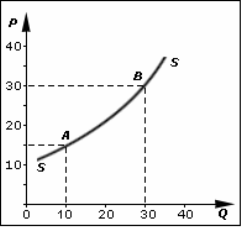
Movement along the supply curve

When the price of goods changes, other factors are kept constant, and the supply of goods changes appropriately. This is due to the direct relationship between the 2. This is known as a change in supply volume. Graphically it causes movement along the supply curve. The change in price causes the supply curve to expand or shrink.

When prices rise and other factors remain constant, the volume of supply increases, which is called the expansion of supply. Graphically, this is represented as an upward movement along the same supply curve.

Conversely, companies tend to reduce supply when prices fall while keeping other factors constant. This is called supply reduction. Graphically, this is often represented as a downward movement along an equivalent supply curve.

Direct relationship with supply

Factors such as the state of technology have a direct relationship with supply. In other words, such factors and changes in supply occur in the same direction. As a result, an increase in such factors leads to a shift in the right direction. Conversely, when such factors decrease, the curve shifts to the left.

Reverse relationship with supply

Factors like the price of other goods tend to be inversely proportional to the supply of goods. Simply put, such factors and changes in supply occur in the opposite direction. Negative changes in such factors cause positive changes in the supply, and vice versa. Virtually an increase in such factors leads to a shift to the left. However, when such factors decrease, the supply curve shifts to the right.

1.6 Market equilibrium and price determination

Introduction to Pricing

Price is the value of buying a finite quantity, weight, or combination of different goods or services. In other words, it also represents the value of goods produced and services provided by such factors of production as land, labour, and capital. Therefore, the determination of prices is very important in the economy.

Introduction to Pricing

Price determination means determining the cost of goods sold on the free market and the services provided. In a free market, the facility of supply and demand determines prices.

The government does not interfere in determining prices. However, in some cases, the government may intervene in determining the price. For example, the government sets a minimum selling price for wheat.

Factors affecting the decision of prices

The factors that affect the pricing of products are:

1] Product cost

The cost of the product is one of the most important factors that affect the price. This includes the sum of fixed, variable and semi-variable costs incurred through the manufacture, distribution and sale of products. Fixed costs refer to costs that remain fixed at all levels of production or sales. For example, rent, salary, etc.

Variable costs are attributed to costs directly related to the level of production or sales. For example, the cost of basic materials, the cost of apprenticeships, etc. Semi-variable costs take into account these costs, which vary depending on the level of activity, but not in direct proportions.

2] Utility and demand

Habitually, end users demand more units of the product when the price is low, and vice versa. On the other hand, if the demand for the product is elastic, then the volume of demand can change significantly if the price fluctuations are small. On the other hand, if there is no elasticity, the change in price will not have a significant impact on demand. In addition, the buyer is ready to pay to the point where he feels that the utility from the product is at least equal to the price paid.

3] Degree of competition in the market

The next consistent factor that affects the price of manufactured goods is the nature and degree of competition in the market. If the degree of competition is low, companies can fix any price for their products. However, if there is competition in the market, we will fix the price, taking into account the price of the replacement.

4] Government and regulatory regulations

Companies that monopolize the market habitually impose high prices on their products. To protect the interests of the people, the government intervenes and regulates the price of goods. For this purpose, it declares some products as indispensable products. For example, life-saving drugs.

5] Pricing purposes

Another consistent factor affecting the price of an item for consumption or service is the purpose of pricing. Maximizing profits, gaining market share leadership, surviving in a competitive market and achieving product quality leadership are the goals of the company's pricing? Generally, companies charge higher prices to cover higher quality and higher costs if backed by the above objectives.

6] Used marketing methods

Various marketing methods such as distribution system, salesman quality, marketing, wrapping type, regular customer service, etc. also affect the price of manufactured goods. For example, if an organization uses elegant materials for packaging a product, the organization will charge an ultra-high amount of revenue.

    Determination of Equilibrium Price

A price that equates demand with supply is called a balanced price.Graphically speaking, the equilibrium price is the point at which the demand and supply curves intersect.There is no unsold stock, and the demand is also a price that can not be met.Therefore, it is also known as market clearing price.

When the equilibrium price and quantity are reached, the stable equilibrium is reached.A stable equilibrium adjusts the disturbance of supply and demand and restores the original equilibrium.

Other things remain the same, but when the price falls below the equilibrium price, demand increases and supply decreases.A shortage of goods occurs, which raises the price to a balanced price.

Similarly, if the price exceeds the equilibrium price, demand will decrease and supply will increase.A surplus of goods occurs,which lowers the price to the equilibrium price.Therefore, the market will restore equilibrium prices by itself.

However, prices are not determined solely by the forces of supply and demand.Other factors such as the price of substitutes, the price of related products, government policy and competition in the market also play an important role in determining prices.

1.7 Elasticity of demand and supply

Subject：

The theory of supply and demand is essential to understanding economics.

It has been argued that a certain relationship exists between price and demand and supply, while others remain constant.

But how much will the demand or supply change if the price changes?A significant increase or decrease in prices may have little effect on demand or supply.

On the other hand, a slight increase or decrease in prices can lead to significant changes in demand or supply.Theoretically, it is impossible to say exactly what happens in such cases.The price and quantity reaction may be different for each product.It is problematic for economists to gather evidence and calculate this relationship.

However, theoretical economists can provide useful guidance for studying this relationship.Elasticity may be a measure of the connection between demand or supply and another variable that affects demand or supply, such as price or income.

Price meaning elasticity of demand：

Price elasticity of demand measures the degree of responsiveness of demand to changes in the price of goods.Therefore, its measurement depends on comparing the rate of change in prices with the rate of change in the resulting volume of demand.

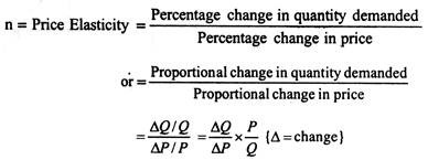
There are slight problems with calculating the rate of change in this way. Depending on whether you move the demand curve up or down, you will get different answers. 1 way to avoid this difficulty is to take the average of 2 prices and 2 quantities in the range you are considering and compare the change in the mean, rather than comparing it with the price or quantity at the start of the change.

The formula for calculating the price elasticity of demand looks like this:

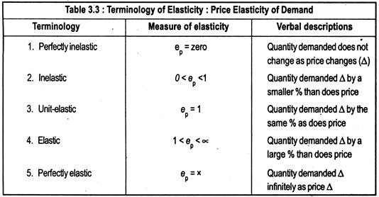
Different kinds of price elasticity：

The range of price elasticity varies depending on whether the 1% change in price is greater or less than the 1% change in demand.

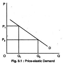
a.Price resilient demand：

If the price elasticity of demand is greater than 1, this is called the price elasticity demand.When the price changes by 1%, a larger response occurs than when the demand changes by 1%: ΔP<ΔQ.

b.Single price elasticity of demand：

In this case, if the price changes by 1%, then the volume of demand changes by exactly 1%.

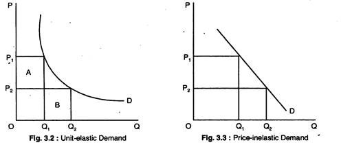
c.Demand without price elasticity：

Thus, a 1% change in price causes a response of less than 1% change in the volume of demand: ΔP>ΔQ.

Elasticity and gradient：

Elasticity and inclination are not the same.It shows that elasticity decreases with Price along a linear demand curve (that is, a straight line with a constant slope).As a matter of fact, the elasticity along the downward-sloping straight demand curve varies numerically from Infinity to zero as you move the curve down.

Therefore, since most goods have both elastic and inelastic ranges, it is necessary to specify the price range when discussing the price elasticity of demand.The only thing that can confirm the elasticity of a straight demand curve is whether it is completely horizontal or completely vertical.The horizontal straight demand curve has infinite elasticity in all quantities, as shown in the figure.

3.4 (a) extreme resilience：

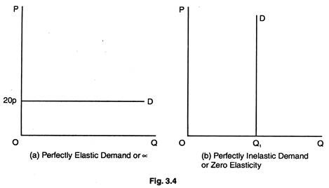
Figure 3.4 (a) shows complete responsiveness. At a price of 20 pence, consumers demand an unlimited amount of the goods in question.Figure 3.4 (b) shows the complete price unresponsiveness.The demand curve is vertical in quantity Q1 units.That is, here the price elasticity of demand is zero.Consumers demand a unit in Q1 for this particular commodity, regardless of the price.

Resiliency and total revenue/total spending：

It is generally believed that the way to increase total revenue or total expenditure is to increase the price per unit. But is this always the case? Is it possible that a rise in unit prices will lead to a decrease in total revenue? The real answer to these questions depends on the price elasticity of demand.

Table 3.1 shows the price of gasoline in pounds, the units requested in Column (2) (per period), the total revenue (P x Q) in Column (3), and the value of elasticity in Column (4). Notice what the total revenue will be for the entire schedule.

As prices rise from £ 1 per unit to £ 1 per unit, they rise steadily. After that, even if the price rises another 1 to 6 pounds per unit, the total revenue will remain constant at 30 pounds. For prices above £ 6, the total revenue actually decreases as the price goes up. Therefore, it is not safe to assume that price increases are always the way to greater income.

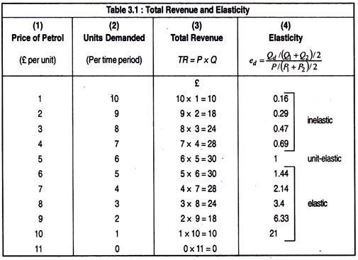
In fact, if the price in this example exceeds 1 pound per unit, then the total revenue can only be increased by lowering the price.

Here, Table 3.1 shows the elasticity, unit elasticity, and inelastic sections of the demand schedule, depending on whether a drop in price increases, keeps it constant, or decreases total revenue. Figure 3.5 shows a graph of total revenue in the elasticity, unit elasticity, and inelastic parts of the demand curve.

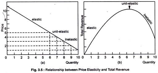
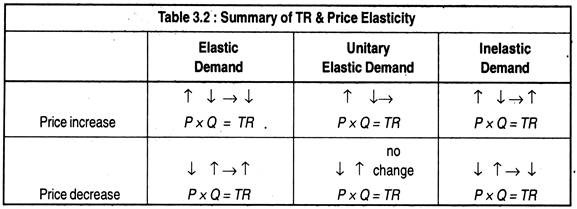
So, there are 3 relationships between 3 types of price elasticity and total income.

a.Price resilient demand：

There is a negative relationship between small changes in prices and changes in total revenue.That means that when prices go down, total revenue increases when companies face price-resilient demand.And if it raises the price, then the total revenue decreases.

b.Unit price-elasticity of demand：

The slightest change in price does not change the total revenue.In other words, if a company is facing unit resilient demand, then even if it raises the price, the total revenue will not change.Even if the price falls, the total revenue will not change.

c.Demand without price elasticity：

A positive relationship between a small change in price and total revenue.That is, when a company is faced with demand without price elasticity, increasing the price increases the total revenue.Lowering the price reduces the total revenue.Figure 3.5 shows areas of the elasticity, unit elasticity, and inelastic demand curves.If the price per unit rises from £ 1 to £ 5, the demand will rise from £ 10 to £ 30, as there is no price elasticity.

However, even if the price is changed from £ 5 to £ 6, the total revenue will remain constant. At £ 30, demand is unit resilient.Finally, if the price rises from £ 6 to £ 11, the total revenue will decrease from £ 30 to £ 0.Clearly, demand is price elastic.This is clearly shown in Figure 3.5.

The relationship between the price elasticity of demand and gross income summarizes several important microeconomics concepts.Total revenue is the product of the price per unit and the quantity of units sold (P x Q).

The demand theory states that along a given demand curve, changes in price and quantity move in the opposite direction, with one increasing and the other decreasing.So, what happens to the product of price and quantity depends on which of the opposite changes will significantly affect the total revenue.This is what the price elasticity of demand is designed to measure the responsiveness of quantities to price changes.

Summarizing the relationship between the price elasticity of demand and total revenue, we can say:

Determinants of price elasticity：

a.Ease of substitution：

The more substitutes are available for the product, the greater the elasticity of demand.For example, the demand for Whole Foods is not very resilient, but if you consider certain foods, you can see that the elasticity of demand is much greater.This is because you can not find an alternative to the whole food, but you can always find an alternative to one type of food.

b.Number of uses：

The more times the goods are used, the greater the elasticity of demand.For example, electricity has many applications such as heating, lighting and cooking.Soaring electricity prices not only make people economical in all these areas, but in some cases could replace other fuels.

c.Percentage of revenue spent on products：

If the price of a packet of salt rises by 50 per cent, for example, from 20p to 30p, it would discourage most people because their share of income is so small.However,if the price of a car rises from £ 4,000 to £ 6,000,even the same percentage rise will have a huge impact on sales.

The larger the percentage of income that the price of a product represents, the more resilient the demand tends to be.

d.Time：

In general, demand elasticity tends to be greater in the long term than in the short term.The period we are considering plays an important role in shaping the demand curve.For example, if the price of meat has increased disproportionately to other foods, you can not immediately change your diet.

Therefore, people will continue to demand the same amount of meat in the short term.But in the long run, people will start looking for alternatives.Whether this is a noticeable effect depends on whether the consumer finds a suitable alternative.It may also be possible to mask the opposite effect.

e.Durability：

The more durable the product is, the more resilient the demand tends to be.For example, if the price of potatoes increases, you can not eat the same potatoes twice.But if the price of furniture rises, you can make the existing furniture last longer.

f.Addiction：

If a product such as a cigarette forms a habit, this tends to reduce the elasticity of demand.

g.Price of other products：

We know that when the price of a product rises, the demand for substitutes increases and the demand for complements decreases.So when demand increases (or decreases) at a certain rate, the elasticity does not change, but when you shift the curve to the right for a certain amount, the elasticity decreases.

In both figures in Figure 3.6, demand is increasing and the demand curve is moving to the right. In Figure 3.6 (A), we can see that shifting the entire curve to the right reduces the elasticity. However, in Figure 3.6 (b), demand is increasing at a certain rate at all prices, and the elasticity remains constant.

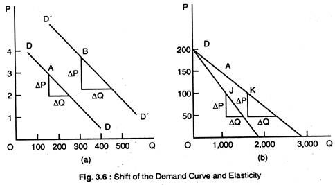
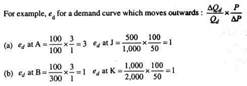
a) when the entire demand curve moves outward, the elasticity decreases.

b) when the demand curve rotates, the elasticity does not change.

Resilience value：

The increase in price (+) causes a decrease in quantity (-), on the contrary, the decree of the value of the answer (-) should always be negative. The coefficients are represented as S by prefixing the equation with a minus sign.So it looks like this:

Arc elasticity：

This is an estimate of the elasticity along the range of the demand curve.

You can calculate both linear and nonlinear demand curves using the following formula:

Arc elasticity of demand：

In this formula, P1 and q1 represent the original price and quantity,and P2 and q2 represent the new price and quantity.

So (P1 + P2)/ 2 is the measure of the average price of the range along the demand curve, and (q1 + q2) / 2 is the average quantity of this range.

Short and long term：

The P elasticity of demand depends on how long consumers can adjust their spending patterns as prices change.The most dramatic price change in the past 50 years-the rise in oil prices in 1973-74-has captured many households with new but fuel-efficient cars.Initially, they expected that the increase in oil prices may not last long.

Then they must have planned to buy a smaller car with more fuel usage.But in countries like the United States, some small cars were still available. In SR, households were stuck.Unless they could realign their lifestyles to reduce car use, they had to pay higher petrol prices.Demand for gasoline has not been resilient.

For a long time, consumers had time to sell large cars to buy fuel-efficient cars or to approach workplaces from far-flung suburbs.Over this long period, they were able to reduce gasoline demand by far more than they initially did.

The price elasticity of demand is lower For SR than for LR if there is room to substitute other commodities.This result is very common.Even if addicted smokers can not adapt to the increase in the price of cigarettes, there will be fewer young people who start smoking, and the number of smokers will gradually decrease.

While responding to the demand for changes in the price of chocolate must be completed within a few months, a complete adjustment to changes in the price of oil and tobacco can take several years.

Use of income elasticity of demand

Income elasticity helps predict patterns of consumer demand as the economy grows and people become richer.Suppose that in the next 5 years real income will increase by 15%.The demand estimate means that the demand for cigarettes will decrease, but the demand will decrease significantly.

The growth prospects of these 2 industries vary greatly.These projections affect companies ' decisions on whether to build new factories and the government's forecasts for tax revenue from alcohol cigarettes.Similarly, as poorer countries get richer, they demand more luxuries such as TVs, washing machines and cars.

Free markets and price controls：

In a free market, prices can be determined purely by force.The d and s curves can be shifted by government action, as if the SC were shifted by a change in safety laws, but the government does not seek to directly regulate prices.

If the price is flexible enough, then the pressure of ED or ES will allow the free market price to bid quickly to the equilibrium level.If effective price controls exist, the market is not free.Price controls can be the lowest price (Lowest Price) or the highest price (highest price).

Price controls are government rules or laws that prohibit price adjustments to clear the market.The price cap makes it illegal for sellers to charge more than a certain maximum price.If the shortage of goods threatens to significantly increase the price, a ceiling may be introduced.High prices are the way of free-market ration goods, where supply is scarce.

This solves the issue of allocation, which leads to the requirement of only a small amount of rare goods, which may be considered unfair and a normative value judgment.High food prices mean difficulties for the poor.In the face of food shortages in the country, the government may impose a price cap on food so that the poor can afford it.

The free market equilibrium is in E.The high price P0 curbed the amount required for undersupplied rations. The P1 price cap succeeds in keeping prices down, but leads to EDAB.It also reduces QS from Q0 to Q1. The price cap at P2 is irrelevant because the free market equation is E.

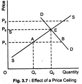
Figure 3.7 shows the food market.The war disrupted food imports. Sc is on the far left of the free market economy.The price P0 is very high. Instead of allowing the free market equation in E, the government imposes a P-cap P1.The sales quantity is Q1 and ED is distance AB.The price cap creates a shortage of supply relative to demand by keeping food prices below equilibrium levels.

The cap price P1 gives the poor more room to buy food, while Ed AB reduces the total amount of food supplied from Q0 to Q1 at the cap price.You need to use rationing to determine which potential buyers will actually be supplied.This distribution system can be arbitrary.

Food is not necessarily sent to the poor, sometimes to the Friends of the suppliers, and sometimes to the rich in line.In the end, keeping food prices down may not help the poor.The cap price is often organized by allocation so that the available supply is distributed fairly, regardless of the tax burden.

The purpose of the price cap is to lower the price of the consumer, while the purpose of the minimum fee is to raise the price of the supplier.An example of a minimum rate is the National Minimum Wage or minimum rate for agricultural products.

Figure 3.8 shows the minimum rate P1 for butter.In the previous example, we assumed that the trading volume would be the smaller of QS and QD at a controlled price, since we cannot force individuals to participate in the market.Another possibility is that the government not only intervenes to set controlled prices, but also buys and sells large quantities of goods to compensate for the purchase and sale of individuals.

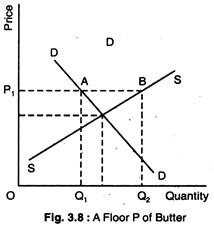
With a minimum fee P1, individuals demand Q1 but supply Q2.If there is no sale or purchase by the government, the transaction volume will be in Q1, whichever is smaller in Q1 and Q2.

However, the government may consent to the purchase of ES AB.This eliminates the need to frustrate both private suppliers and private consumers.Because European butter prices are set above the free market equilibrium price as part of the CAP, European governments were forced to buy large quantities of butter that would otherwise not have been sold at a controlled price.Hence the famous mountain of butter.

At the lowest rate, the supply of P1 is Q2,but the demand is Q1. Only Q1 will be traded. By purchasing ES ab, the government can satisfy both suppliers and consumers with the price of P1.

Income elasticity：

We know that there are several determinants of product demand.In the past, we have been concerned about how demand will change as prices change.1. Another important determinant of demand is Income (Y).The response of demand to changes in income can also be measured.

Income elasticity of demand measures the degree of responsiveness of the volume of demand for a product to changes in income.Income elasticity of demand

Ey =rate of change in demand/rate of change in income

 or  x   

Where Y is income

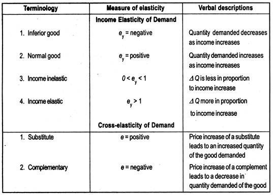
For most commodities, income elasticity will be positive, since an increase in income will lead to an increase in demand.Income elasticity has the same subdivision as price elasticity.Thus, the commodity can be income elasticity, income inelastic, and unit income elasticity.

Virtually all goods have a negative price elasticity.However, income elasticity can be both positive and negative.Goods with a positive income elasticity are usually called goods.Goods with a negative income elasticity are called defective products.For them, the increase in income is accompanied by a decrease in the volume of demand.Ordinary goods are much more common than inferior ones.

Cross-elasticity：

The responsiveness of the volume of demand for 1 commodity to changes in the price of another commodity is often of considerable concern.This type of responsiveness is called cross-elasticity of demand.

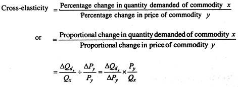
Cross elasticity varies from minus infinity to plus Infinity.Complementary goods have a negative cross-elasticity,and alternative goods have a positive cross-elasticity.

Supply elasticity：

Much of what we have said about the elasticity of demand also applies to the elasticity of supply.The definition of the elasticity of supply is very similar.

The elasticity of supply measures the degree of responsiveness of the supply to changes in price.

Thus, the elasticity of the supply can be written as follows:

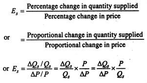
This looks the same as the formula for the elasticity of demand.However, remember that the price elasticity of demand is always negative.However, the supply curve is tilted upward from left to right, so the price elasticity of the supply is usually positive.Except in the case of a supply curve that bends backwards,in which case it will have a negative elasticity.

Feed elasticity labeling：

As shown in Figure 3.9, there are 3 cases of supply elasticity. SS is a fully elastic supply curve, S ' S 'is a zero elastic (or completely inelastic) supply curve,and OS' is a unit elastic supply curve.The linear supply curve passing through the origin has 1 elasticity, regardless of the steepness of the curve.

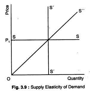
Supply elasticity of demand

Supply and demand elasticity#15.Price elasticity of supply and length of adjustment time：

We already know that the longer the adjustment takes, the greater the price elasticity of demand.The same proposition applies to supply.

The longer the adjustment takes, the higher the price elasticity of the supply curve.

1.The longer the time allowed for adjustment, the more companies can find ways to increase production in the industry.

2.The longer it is allowed, the more resources may flow into the industry through the expansion of existing companies.

Therefore, we talk about the short-term and long-term price elasticity of supply.A short term is a period during which a full adjustment has not yet been made.In the long term, it is the period when the enterprise was able to fully adapt to changes in prices.

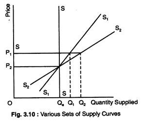
Set of different supply curves

You can view the entire set of supply curves similar to what you did for demand.In Figure 3.10, if nothing can be done in the short term, the supply curve is vertical SS if the price is Pe and the supply quantity is Qe.

If the given price goes up to P1, there will be no short-term change in the supply volume.It remains in Qe.If you adjust the same time, the supply curve will rotate from price Pe to S1S1.The new quantity supplied shifts out to Q1 at P1.Finally, the long-term supply curve is shown by S2S2.The supply will increase again in P1 to Q2.

Determinants of supply elasticity：

The elasticity of supply is very important in economics.

There are several factors that affect the elasticity of supply, as well as demand.

(a)Time：

This is the most important factor, as we have seen how elasticity increases over time.

(b) factor mobility：

The ability to easily move production factors from one application to another affects the elasticity of supply.The higher the factor mobility, the greater the elasticity of the supply.

(c)natural constraints：

Nature imposes restrictions on supply.For example, if you want to produce more vintage wines, it will take years to mature to become vintage.

(d)risk-taking：

The more entrepreneurs try to take risks, the greater the elasticity of the supply. This is partly affected by the system of incentives in the economy. For example, if the marginal tax rate is very high, the elasticity of the supply may decrease.

(e) cost：

The elasticity of supply largely depends on how costs change as output changes. If unit prices rise sharply as output increases, the stimulus to expand production in response to price increases is immediately suppressed by the increase in costs incurred as output increases. In this case, the supply is not quite elastic.

SOn the other hand, if the unit price increase is slow with the increase in output, if the profit increases due to the increase in price, the supply will increase significantly before the increase in cost stops the increase in output.In this case, the supply tends to be quite resilient.

1.8 Application of demand and supply.

The analysis of price determination from the point of view of supply and demand is of great theoretical importance, as well as some practical application in the economic life of the country. This supply and demand analysis has been used to explain the effects of price controls and rationing, minimum price manipulation, tax consequences, and several other economic issues and policies. This current article describes some of these applications of supply and demand analysis.

Market mechanisms are allowed to function without government interference. However, governments in a modern mixed economy interfere with the functioning of the market system, which affects prices to promote social welfare, when it is felt that the free work of the market does not produce the desired result.

The government can interfere with the work of the economy in 2 main ways.The first government fixes the highest price (often called the lowest price) or the lowest price (often called the lowest price).Food grain price controls, rent controls, are examples of fixing the maximum price or price cap where the seller cannot charge the price.The agricultural product price support program is an example of fixing the lowest price to guarantee the lowest reward price to farmers to protect the interests of farmers.
The 2nd way for governments to interfere with prices and market systems is to function through markets.In the second way, the government can tax goods or provide subsidies.These taxes and subsidies affect the supply and demand curve of the market, which determines the price of goods and services.

Imposing heavy excise taxes on tobacco and other drugs or providing subsidies to agricultural products are examples of government interference through markets.Below, we will discuss both types of government intervention in the functioning of the market and begin our analysis from the imposition of price controls and government distribution.

Price controls and rationing：

During the war, the imposition of price controls was very common and was introduced by several countries during the Second World War.Even in peacetime, commodity price controls were introduced in some countries to help the poor against inflation.

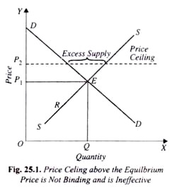
Under price control, the highest price of the goods is fixed,beyond which the seller can no longer be charged by the consumer.Price controls are imposed or the price cap is below the equilibrium price.This is because if the price cap is set above the equilibrium price, which balances supply and demand, it has no effect, that is, it is not binding.

Consider the balance between supply and demand at price P1 (figure 25.1).At this equilibrium price, both the buyer and the seller are satisfied, the buyer gets the amount of goods they want to buy at this equilibrium price, and the seller sells what they want to sell at this price.Therefore, the price P2, which is higher than the price P1 set by the government, has no effect.

If you notice that the equilibrium price of the goods is too high, and as a result some buyers are dissatisfied, the government may pass a law that fixes the highest price of the goods to a certain level, because they have no means to pay for it.It is below the equilibrium price.

Now,at a price lower than the equilibrium price, the demand will be more than the supply, resulting in a shortage of goods.Some consumers, who are willing to buy at that price, can not be satisfied.The buyer, if allowed, will raise the price to an equilibrium level.

But under government price controls, prices cannot move freely to equalize demand and supply.Therefore, if the government intervenes to determine the highest price of goods, the price loses the vital function of the ration apparatus.

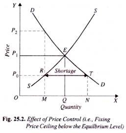
Price controls and the problems caused by them are shown graphically in Figure 25.2.Here, the curves of sugar supply and demand, DD and SS are shown.As you can see from this figure, the supply and demand curve intersects at Point E, so OP1 is the balanced price of sugar.Assume that this balanced price of sugar is so high that many poor people can't get the amount.Of it.Therefore, the government intervened and fixed the maximum price of sugar at the level OP1 below the equilibrium us OP0.As can be seen from figure 25.2, the demand for the managed price OP0 exceeds the supply.At price OPo, producers offer to supply p0r amount of sugar, but consumers are ready to buy p0t amount of sugar.As a result, there will be a shortage of sugar, which is equivalent to the RT amount, and some consumers will be dissatisfied.

In the absence of government intervention to fix the maximum price to the OP (j level), excess demand equal to RT will cause the price to rise to the equilibrium level OP, where the demand is equal to the supply.However, under price control, it is punishable under law by the government to charge a price higher than the legal maximum price OP0.

Therefore, the supply OM available at a fixed price OPQ must be allocated or allocated among consumers in some way.Ration can take many forms.Rationing the available supply OM this task can be done by the producer or the seller himself.

Sellers can adopt the principle of"first come, first served" and distribute the supply of available sugar to people who are in line first before the store.Therefore, this distribution system is called queue distribution.

The 2nd way to allocate or allocate the supply of the missing goods is to distribute the goods on the basis of the so-called"allocation according to the seller's preferences".Under this, the supply of available goods is sold to regular customers at controlled prices.We may also adopt a policy of selling supplies available to buyers belonging to a particular caste, religion, color, etc. but not to other buyers.

If the government does not like the distribution of goods between the population on a"first come, first served basis"or arbitrary allocation by the seller's preference, it may introduce coupon rationing of goods.

In the coupon distribution system, consumers are given just enough ration coupons to purchase the available quantity of goods.The number of ration coupons issued to a family depends on the age, gender, number of family members or other criteria considered desirable.

Black market：

What is noteworthy is that price controls with or without ration are likely to trigger a black market for goods.The black market means that the producer or seller sells the goods at a price higher than the managed price.

As mentioned earlier, at the managed maximum price, fixed below the equilibrium price, the volume of demand exceeds the volume of supply, resulting in a shortage of goods.Therefore, it is clear that some buyers of goods are not completely satisfied, because they can not get the quantity of the goods they want to buy at a controlled price.

Therefore, they are ready to pay a higher price to get a larger amount of goods, but they can only do so on the black market.Sellers will also be interested in selling goods, at least their quantity, at a higher price on the black market, since they can get a greater profit.

Even if coupon rationing is introduced, there is pressure on the development of the black market.This is because consumers are willing to buy more goods than are available at a controlled price, whereas ration distributes only the available quantity of goods.Therefore, consumers who want to procure a larger volume than the ration are ready to pay a higher price in order to get some volume on the black market.

There is enough evidence in India and abroad to confirm forecasts based on the analysis of supply and demand.After World War II, when Price Controls and rationing systems were introduced for some of the missing goods, the black market developed despite punitive measures by the authorities.

Rent management：

Rent control is another 1 example of the highest price the government fixes on the rent of a housing unit.Under rent control, the government will fix the monthly rent per standard-sized residential unit, which is lower than the aquarium rent, which would otherwise be popular in the market.

The maximum rent set by the government assists tenants who generally belong to low and middle income groups and are intended to prevent exploitation by wealthy landlords who charge rent determined in a very high market.Demand for rental housing tends to be relatively higher than supply, so the market-determined equilibrium rents happen to be higher.

In several important cities such as New York, London, Mumbai and Delhi.The government imposes rent controls to help low-and middle-income people by securing rental housing at Fair Rent. The Delhi Rent Management Act of 1958 was amended by the new rent Management Act which was recently passed in Delhi under the 19

The law specifies the monthly rent for some standard-sized housing units, where landlords cannot charge rent.Also, the landlord can not easily evict the tenant, except for the conditions established by law.However, it is important to understand both the short-term and long-term effects of rent management.

Economists often point to the negative effects of rent control and have the view that it is a very inefficient way to help poor middle class people.The negative effects of rent control are evident only in the long run, as it always takes time to build new housing units/apartments and also time for tenants to adapt to housing accommodation available for rent and rent.

Therefore, the long-term effects of rent management are different from short-term ones.In the short term, landlords have an almost certain number of residential units/apartments to pay rent.Therefore, the supply curve of rental units is not resilient in the short term.

On the other hand, people looking for rental housing will not have much reaction in the short term, as it will always take time to adjust the placement of housing.Therefore, even the demand for rental housing in the short term is relatively less resilient.

Effect of short-term rent management

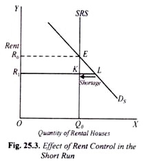
Therefore, the short-term supply curve for residential units is not entirely resilient in the Q0 number of leasable residential units. Ds is a short-term demand curve, which is also relatively less resilient.If left to market forces at will, a rent equal to R0 is determined,creating an equilibrium between supply and demand.

Suppose that R0 is too high to be paid by poor and middle class people.To help them, the government will fix the rent cap on R1.From figure 25.3, we can see that in R1 people demand RXL housing units, whereas their supply remains R1K or OQ1.In this way, short-term housing supply and demand is not resilient, and the shortage by rent management is small, KL housing shortage has occurred.The main effect of short-term rent management is to lower rent.

In the short term, landlords will not be able to contribute much to the reduction of rent by management, but further investment by landlords in the construction of houses and apartments will decrease, and in the long term the supply of rental housing will decrease.

In addition to this, landlords do not spend a set of money and maintenance costs for rental housing when the rent goes down.These steps eventually lead to a decrease in the quality of rental housing and apartments.

Therefore, in the long run, rent control has a significant impact on the availability or supply of rental housing and its volume.From figure 25.4, we can see that when the managed rent or1 becomes lower, the demand for rental housing increases to OQ2 and the supply of rental housing decreases to OQ1.

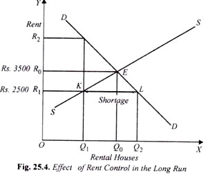
As shown in Figure 25.4, a significant shortage of rental housing equivalent to Q1Q2 or KL occurs when the lower managed rent or1 is fixed. 。In the long term, the higher the supply and demand elasticity of rental housing, the greater the shortage of rental housing due to the enforcement of the rental management law.

Effect of long-term rent management

It should be noted that this shortage of rental housing represents a situation of excess demand for rental housing.The key question is whether we can effectively implement the fixing of the maximum rent, which is lower than the equilibrium rent, in the event of excessive demand or a shortage of rental housing.

Of course, no one can charge rent higher than the openly or explicitly managed rate.However, the emergence of a situation of excessive demand or a shortage of rental housing tends to put upward pressure on the rent they actually receive.

Due to the excessive demand situation, landlords have devised various ways to circumvent the rent control law and charge higher actual rent.Consider figure 25.4.Here we can see that the rental housing supply is OQ1, with the managed rent OR1 for rental housing.In addition, tenants of the oq rental housing unit

In addition, as a condition of rental, the landlord may require the tenant to make expensive accessories or perform expensive woodwork in the rental house, in addition, to pay for the repair and maintenance of the rental housing unit.All these ways of circumventing the Rent Control Act have been observed.

Unless the law explicitly prohibits such practices, they will work and have the effect of nullifying rent control policies.That is, the tenant explicitly pays the managed rent or, but the additional expenditure and required payment could be R ^ R0 per 1 month, and the actual effective monthly rent would be balanced rent or0.

As is clear from the above, the result of rent control, as with other price controls, is the emergence of shortages.However, if there is a shortage of rental housing, if you can not get it, we will arrange another housing.

They may decide to live in other cities or satellite cities that are not subject to rent control.In addition, disappointed seekers of rental housing may turn to the construction of their own private housing.But this requires a lot of finances, which must be arranged by them.

Lowest support price：

Price controls were considered when the government set a price cap (that is, the highest price) so that it would not rise to the equilibrium level.For many agricultural products, the government's policy was to fix the lowest rates, that is, the lowest support prices above the equilibrium levels, which are considered low and unpaid for farmers.

In the case of price controls or price cap fixing, the government simply announces the maximum price that the producer or seller of the product cannot charge the price if it exceeds it, but in the case of the minimum support price, the government becomes an active buyer of the product.Market.

Not only in India, but also in developed countries such as the United States, agricultural product price support policies have been adopted to provide farmers with reasonable prices and increase their income.Impact of imposing a minimum support price on wheat, an important agricultural product

India is shown in Figure 25.5.Here, the wheat demand curve DD and the supply curve 55 intersect at point E.So, if the price of wheat can be determined by the free work of the supply and demand of wheat, then the equilibrium price will be the OP and the equilibrium amount.It is the OQ that is determined.

Lowest support price for agriculture

Here we assume that the equilibrium price OP (=500 rupees per quintal) determined by this free market is considered unpaid and does not provide farmers with an incentive to produce wheat or expand production.Therefore, in order to promote the interests of farmers, the government will intervene and fix the minimum support price OP (1 Rupees per 550 quintals) for wheat.

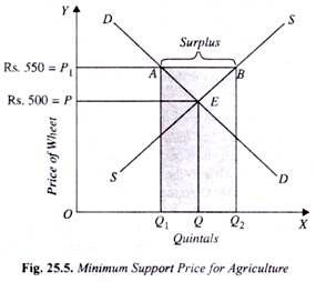
From figure 25.5, we can see that at the price of wheat, the demand for wheat decreases to OQ1 (=P1A).On the other hand, at higher prices OP1 farmers will expand their output and supply more quantities of oq2 (=P1B) wheat.So, with the minimum support price OP1, the amount of wheat supplied by the fan exceeds the amount demanded by the consumer in the market.

This means that imposing a minimum support price for wheat higher than the equilibrium price OP will lead to the emergence of a wheat surplus equal to AB or Q1Q1.If the government does not buy this surplus, this tends to push down the price of wheat.

Therefore, in order to guarantee the farmers the lowest price of this wheat OP (=550 rupees per quintal), the government must purchase the full amount of the surplus AB or Q1 from the farmers.It should be noted that in order to buy surplus Q1Q2 from farmers, the government must spend equal to OP1 X Q1Q2, that is, the area Q1ABQ1.This expenditure on the purchase of wheat surpluses may be financed by people's taxation.

From the above,under the minimum support price OP1, farmers sell to the government the amount of oq1, the amount of wheat on the free market and Q1Q2.In the equilibrium price OP and quantity OQ determined by the free market, the total income of the peasant will be equal to the area OPEQ.

At present, the minimum support price is equal to OP, the total sales volume is equal to OQ2, and farmers ' income has increased to OP1BQ1.Therefore, the minimum support pricing policy has brought great benefits to farmers both in terms of the price they receive for their products and the income they can earn.

The big question facing the government is how to dispose of the surplus purchased from farmers at a higher minimum support price.If the government sells it on the market, the price of wheat on the market will fall and the purpose of the support pricing policy will be undermined.

Alternatively, the government may store the surplus, in which case the government will bear the storage costs.Besides, wheat and other edible grains will rot when stored in storage boxes for a long time.Thus, creating surpluses requires valuable resources such as Labor, fertilizer, irrigation and other inputs, but often rot in government warehouses.

1. In the United States, one of the key ways to dispose of surplus is to give surplus to developing countries as food aid.But this food aid is not without problems.American food aid to developing countries tends to push down the price of food grain in these countries, and thus has harmed the interests of farmers in these developing countries.

In India, the Food Authority of India, on behalf of the government, procures surplus wheat and rice production resulting from a fixed minimum or support price for wheat and rice.The Indian Food Authority then stores it in warehouses.

Surplus food is then used for distribution through the Public Distribution System (PDS) at lower rates.Because the government procures these edible grains at a higher rate and sells them to consumers at a lower issue price, the government must subsidize the consumption of edible grains and incur a food subsidy of several thousand kroner each year.

In addition, surplus food procured by the government will also be used to feed workers under the"food for work"program, Jawahar Rozgar Yojana, and other special employment schemes launched in India.Part of the wages are paid in food, part in the form of money.

At present, the food surplus of wheat is also a problem in India.The good monsoon over the past 6 years has brought food production to a significant amount,and the government has purchased the surplus at a higher procurement price.

The surplus with the government is growing. In 2003-6, it was estimated at about 5,000 tons.Meanwhile, off-takes from the public distribution system have declined.There is a risk that these surplus food will rot in the warehouses of the Indian Food Authority.Therefore, the Indian government decided to export wheat.

It should be noted that in the government of India, procurement or support prices for wheat and rice are increasing year by year.This raises food costs in every sector of the economy and that must lead to higher prices overall.Thus, the increase in wheat and rice procurement prices has become a key factor that has created inflationary pressures on the Indian economy.

The key results of the price support policy are summarized below.-

1.When the minimum support price for agricultural products is fixed at a level higher than the equilibrium price, the price paid by consumers who buy from the open market increases.This is due to the decline in the supply of agricultural products on the open market as a result of the government's purchase of agricultural products from farmers.

2.The fixation of the minimum support price (that is, the minimum fee) leads to the emergence of a surplus of wheat, which the government must buy from farmers.This is very evident from the Indian experience, where the fixation of a higher minimum support price (MSP) has resulted in a mountain of edible grain with the Indian Food Authority.

3.Taxpayers pay more taxes to cover the government's wheat purchase and storage costs.

4.The big question is how to dispose of the surplus purchased from farmers.There are several ways to dispose of the raised surplus.One way is to sell it at subsidized rates to people below the poverty line through the Public Distribution System.Secondly, the surplus can be used to pay part of the wages in terms of food grain, under the"food for work" program.Third, surplus food can be provided to other countries as foreign aid or exported.

5.The income of the peasants increases as a result of which the minimum support price is fixed at a level higher than the free market equilibrium price.As a result of price support, they receive higher prices than they spread in the free market, and also produce and sell more than before.They sell part of their larger production in the market and part to the government.

Incidence of indirect taxes：

An important use of the supply and demand model is to explain the issue of the occurrence of indirect taxes, such as Excise and excise taxes.The occurrence of taxes means who bears the burden of taxes.

For example, if a product is subject to consumption tax, the question is whether the producer bears the tax burden, the consumer who buys the product, or whether the consumption tax money is borne by the producer and the consumer.Limited to the description of the incidence of indirect taxes, that is, taxes imposed on either the production, sale or purchase of goods.

It is worth noting that the price of goods is determined by supply and demand only if full competition is winning in the market.The supply curve of goods is inclined upward, as it is assumed that the marginal production costs will increase with the increase in the volume of production of the enterprise.

An upward sloping supply curve means that producers will offer more sales volumes in the market as the price of goods rises.If the goods are not taxed, the seller or producer receives the full amount of the price.

Well, if the consumption tax is equal to rupees.For 5 per unit, the supply price of each unit of the quantity sold on the market will rise Rs. 5.In this case, the producer receives the amount from the market price minus the amount of tax per unit.

So, if the producer receives a price for the same amount as before the excise tax, then the supply price for each unit of goods sold will increase by the full amount of the tax.This means that the supply curve of goods shifts upward by the amount of tax as a result of the excise tax being imposed.

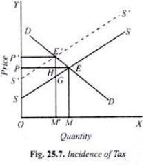
Consider figure 25.7, which shows the curve of supply and demand for goods.Before imposing indirect taxes, the equilibrium price (OP) and the equilibrium amount (OM) are determined because the supply and demand curves intersect at Point E.

Now suppose that a sales tax equal to the amount of SS is imposed on the goods.As explained above, the imposition of excise duty shifts the supply curve vertically upwards.A new supply curve S’S ’is drawn to represent the supply position after the consumption tax is imposed.From figure 25.7, we can see that the new supply curve S’S ’intersects the specific demand curve DD at Point E.

Tax consequences

So, as a result of the imposition of excise taxes, the price of goods rose from OP to OP.This means that consumers will have to pay a higher price for the goods by the amount of PP than before.Obviously, the tax burden borne by consumers is equal to PP ' (=E'H).This is the consequence of the tax imposed on consumers.

From this figure we can see that the quantity sold in the market will be OM, and the government will receive E'g per unit of that as tax. E'h is paid by the consumer,so the remaining tax equal to the amount of GH per unit is borne by the producer or seller.

Thus, part of the tax is passed on to consumers at a higher price,and part is borne by the producers themselves.It is worth noting that the tax consequences borne by producers and consumers depend on the elasticity of demand and supply.The lower the elasticity of demand, the greater the tax consequences that consumers bear.

If the demand for goods is not completely resilient, the entire burden of the goods tax falls on the consumer.This is shown in Figure 25.8.In this figure, the demand curve DD is a vertical straight line indicating that the demand for the goods is completely inelastic.

As a result of the intersection of supply and demand curves, the price OP is determined.When a tax equal to SS ’is imposed on the goods here, the supply curve shifts vertically upwards to the dotted position S’S’.We can see that the new supply curve S'S 'intersects the demand curve DD at the point EE'and the new equilibrium price OP 'is determined.

From figure 25.8, we can see that in this case the price of the product is increasing by PP 'or EE'.This is equivalent to the full amount of tax SS'.This means that producers pass the full amount of tax to consumers, and they themselves do not bear any accruals.Therefore, in the case of completely unsolicited demand, the entire tax return will be on the consumer.

Conversely, as shown in the DD curve in Figure 25.9, if the consumer's demand for the quantity is fully elastic, then the price will not rise if tax is imposed on it.In this case, the full responsibility is borne by the manufacturer or seller.From figure 25.9, we can see that the equilibrium price does not change at the level OP as a result of the indirect tax on the amount of SS ’and the resulting upward shift in the supply curve to S’S’.In this case, the consumer will not bear the burden of taxes, since the price has not gone up.Therefore, the entire tax return will be on the producer, or in the case of a completely resilient demand, the seller.

So, as a result of the imposition of excise taxes, the price of goods rose from OP to OP.This means that consumers will have to pay a higher price for the goods by the amount of PP than before.Obviously, the tax burden borne by consumers is equal to PP ' (=E'H).This is the consequence of the tax imposed on consumers.

From this figure we can see that the quantity sold in the market will be OM, and the government will receive E'g per unit of that as tax. E'h is paid by the consumer,so the remaining tax equal to the amount of GH per unit is borne by the producer or seller.

Thus, part of the tax is passed on to consumers at a higher price,and part is borne by the producers themselves.It is worth noting that the tax consequences borne by producers and consumers depend on the elasticity of demand and supply.The lower the elasticity of demand, the greater the tax consequences that consumers bear.

If the demand for goods is not completely resilient, the entire burden of the goods tax falls on the consumer.This is shown in Figure 25.8.In this figure, the demand curve DD is a vertical straight line indicating that the demand for the goods is completely inelastic.

As a result of the intersection of supply and demand curves, the price OP is determined.When a tax equal to SS ’is imposed on the goods here, the supply curve shifts vertically upwards to the dotted position S’S’.We can see that the new supply curve S'S 'intersects the demand curve DD at the point EE'and the new equilibrium price OP 'is determined.

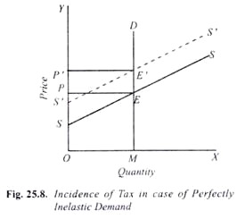
From figure 25.8, we can see that in this case the price of the product is increasing by PP 'or EE'.This is equivalent to the full amount of tax SS'.This means that producers pass the full amount of tax to consumers, and they themselves do not bear any accruals.Therefore, in the case of completely unsolicited demand, the entire tax return will be on the consumer.

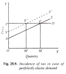
Conversely, as shown in the DD curve in Figure 25.9, if the consumer's demand for the quantity is fully elastic, then the price will not rise if tax is imposed on it.In this case, the full responsibility is borne by the manufacturer or seller.From figure 25.9, we can see that the equilibrium price does not change at the level OP as a result of the indirect tax on the amount of SS ’and the resulting upward shift in the supply curve to S’S’.In this case, the consumer will not bear the burden of taxes, since the price has not gone up.Therefore, the entire tax return will be on the producer, or in the case of a completely resilient demand, the seller.

Tax consequences in case of completely unsolicited demand

It should be noted that the less resilient the demand for goods, the greater the increase in prices that consumers pay, and vice versa.To illustrate this clearly, figure 25.10 shows 2 demand curves.1 is inelastic and the other 1 is relatively elastic.At the same point F, the supply curve SS intersecting 2 demand curves DD and D'd is drawn.

The sales and purchase quantities before tax are OM,and the price of the goods is OP1.Here, when a sales tax is imposed, the supply curve shifts upwards to S ' S ’by the amount of tax per unit imposed.From figure 25.10, we can see that the new supply curve S’S ’intersects the inelastic curve DD at the point S, which determines the equilibrium price OP.

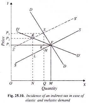
In the case of this inelastic demand, prices are rising only by p1p3, which is a burden on consumers.Where the new supply curve S ' S ' intersects the relatively resilient demand curve D'd’at the point R at which the market price OP2 is determined.

Thus, in the case of an elastic demand curve D'd’, the price increase as a result of the same tax will be equal to P1P3, which is less than p1p2, which is borne by the consumer in the case of unsolicited demand.Therefore, how much the tax return will fall on the consumer depends on the elasticity of demand for the goods in question.

Predictions about the tax consequences borne by consumers and producers have generally been found to be true in real-world situations where goods subject to tax are sold under competitive conditions.

Stabilization of prices and incomes in agriculture：

The analysis of supply and demand has an important use in understanding agricultural issues and assembling appropriate policies to stabilize agricultural prices and incomes.The nature of the supply and demand of agricultural products is also unique.

The demand for agricultural products is relatively resilient.This means that the amount required for agricultural products will hardly change, regardless of whether prices go up or down.This is because agricultural products belong to the"necessities group", which can not be let go, and in times of hardship inferior products are replaced by superior ones, or in periods of prosperity there are no good substitutes, except for that.The peasants themselves may give up the consumption of millet for inferior products,for example, wheat or rice.As can be seen below, the relatively unsolicited demand curve of agricultural products has a significant impact on the price and income of agricultural products.

The supply of agricultural products also has a unique nature.This is because the production of agricultural products is subject to very large fluctuations due to natural factors beyond human control.

For example, if the monsoon fails in India or fails in time, agricultural production will fall considerably.On the other hand, when the monsoon is favorable, a good harvest occurs, resulting in an increase in the supply of agricultural products on the market.

Similarly, the ingress of pests and insecticides, the occurrence of floods are other natural factors that cause unplanned fluctuations in agricultural production.Unplanned fluctuations in agricultural output due to natural factors have a significant impact on farmers ' prices and incomes.

Now, I will explain below how the supply and demand of agricultural products determine the price of agricultural products, and how unplanned fluctuations in agricultural products affect the price and income of agricultural products.

SThe effect of unplanned fluctuations in agricultural supply on prices：

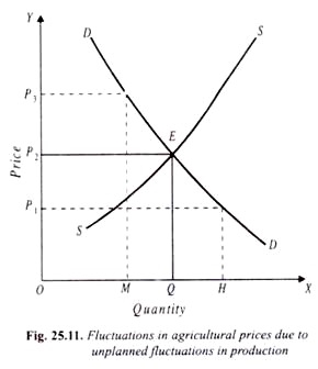
Consider figure 25.11, in which the relatively unsolicited demand curve DD of agricultural products is drawn. SS shows the supply curve according to the planned output and sales by farmers at different prices.Now, from figure 25.11, you can see that this supply curve, SS, showing planned production at different prices, intersects the demand curve specified at Point E.

Therefore, the price OP1 and the transaction quantity OQ are determined. OQ is the normal quantity produced and sold at price OP1.If, due to some natural factor, 1 year of production falls on OM, then there will be a shortage of goods equal to the quantity of QM.

The lack of production of this commodity leads to an increase in the price of agricultural products.From figure 25.11, we can see that using OM as a supply of agricultural products increases the price of goods to OP1.With the increase in price to this OP, the amount of demand will be equal to the available output OM.

Here, suppose that unplanned production of agricultural products increases to OH due to favorable weather.This will be greater by QH than the normal output OQ.Thus, as a result of an unplanned increase in output, a surplus is generated, which is equal to the volume of QH.

This surplus will lead to a fall in prices for agricultural products.From figure 25.11, we can see that if we use OH in the production of agricultural products, the price will fall to the level of OP1, and the demand will be equal to the level of available production.

Thus, we can see that as a result of unplanned fluctuations in agricultural products, prices for agricultural products fluctuate considerably.It is also clear that unplanned fluctuations in agricultural production lead to changes in prices in the opposite direction to changes in output.That is, the higher the volume of production, the lower the price, and vice versa.

The effect of unplanned fluctuations in production on the income of farmers：

At present, these unplanned changes in agricultural production and accompanying price changes have significantly changed the income that farmers earn.In this connection, the elasticity of demand for agricultural products plays an important role, since it determines the change in the income of farmers.

If the demand for agricultural products is a single elasticity, the change in prices brought about by the change in unplanned fluctuations in agricultural products will offset the production effect, and as a result, the income that farmers earn will remain unchanged.

On the other hand, if the demand for certain agricultural products is elastic, an unplanned increase in agricultural products will only cause a slight drop in prices, and the income by farmers will increase.

On the other hand, if the production of agricultural products decreases in the face of the elasticity of the demand curve, the price increases will be less compared to the decrease in the production of agricultural products, resulting in a decrease in the income of farmers.

If the demand for agricultural products is not resilient (that is, less than 1), the income of farmers decreases with a fall in prices due to an unplanned increase in production, while the income of farmers increases with a rise in prices.It was brought on by an unplanned drop in production.

Thus, we reach the following forecasts for changes in income with changes in production.

1.Unplanned fluctuations in agricultural production can cause significant changes in the income of farmers through changes in prices.

2.If the demand for agricultural products is elastic, an unplanned increase in production will increase the income of farmers, and an unplanned decrease in production will decrease the income of farmers.

3.If there is no elasticity in the demand for agricultural products, the increase in their output will reduce the income of farmers.

4.The greater the divergence (in which direction) from the unity of the elasticity of demand, the greater the fluctuations in the income of farmers following unplanned changes in agricultural production.

There is a lot of empirical evidence from the real world to confirm the above conclusions based on the analysis of supply and demand applied to agriculture.Unplanned changes in the production of agricultural products occur often.

Since the price of most agricultural products is determined by a fully competitive market, there is generally a significant change in the price of agricultural products.In addition, the demand for most agricultural products is not very resilient, so fluctuations in production cause very large changes in prices.The unsolicited nature of demand for many agricultural products causes a unique phenomenon - "poverty in the rich".

This happens when there is a good harvest, which is expected to bring prosperity to farmers, but this does not happen because of the lack of elasticity of demand.A good harvest leads to a very large decline in prices, and because of the unsolicited nature of demand, the income obtained by farmers falls.Therefore, mass production does not raise the peasant, but lowers the income of the peasant.

On the contrary, if the production of crops falls slightly due to bad weather, the income of farmers increases.This is due to the fact that the price increases significantly due to a decrease in crop production, and the income of farmers increases due to the lack of elasticity of demand.

From the farmer's point of view, lower production at a higher price is better than larger production at a lower price.But it's a bigger production at a lower price than consumers want.Thus, the interests of farmers and consumers are not consistently at odds with each other、

Stabilization of prices and income of agricultural products：

The demand and supply of agricultural products have a unique nature, so if left to the free market, the price of agricultural products and the income of farmers will fluctuate greatly.These agricultural fluctuations are caused either by unplanned changes in agricultural products or by changes in demand for agricultural products.

To protect the interests of farmers, governments of many countries have intervened to stabilize prices and incomes of Agriculture.The government may also aim to increase farmers ' incomes.However, as can be seen below, the policy of stabilizing agricultural prices and the policy of increasing the income of farmers are often contradictory.

Below we will analyze the stabilization of prices and incomes of agricultural products, and policies to increase the income of farmers, in the context of unplanned fluctuations in the supply of agricultural products.A similar analysis can be made if demand changes.

The stabilization of Agricultural Prices is shown in Figure 25.12.Here, the curve of supply and demand for certain agricultural products is drawn.The supply curve (SS) depicted in Figure 25.12 shows the amount that farmers plan or want to produce at each given price.Now, if production can be reliably planned, SS represents the normal supply curve.

Then, this supply curve SS intersects the demand curve DD given at Point E,where the free market price is settled at equilibrium level OP2,and OQ represents planned production traded at equilibrium price OP2.

Stabilization of peasant income by the government

However, actual output is different from the generally planned equilibrium output OQ due to weather fluctuations.Assume that the actual output fluctuates around OQ between the amounts of OL and OH. If we consider OL as the actual supply and the demand curve DD, then the free market price will settle to OP3, OH as the actual supply, and the free market price will settle to OP1.

Therefore, with actual production fluctuations between OL and OH, free market prices fluctuate between OP3 and OP1.Farmers ' income fluctuates due to fluctuations in actual output and accompanying price fluctuations.

Since the income of the peasant is equal to the output multiplied by the price,in the planned production OQ, the income of the peasant is equal to the area of the rectangular OP2EQ.Similarly, with OL as the actual production volume, OP1 as the price, the farmer's income will be equal to the area of rectangular OP3 KL,OH as the actual production volume,OP as the free market price,the farmer's income will be as follows.Rectangle OP, TH.Therefore, fluctuations in real production and accompanying changes in free market prices cause fluctuations in the income of farmers.

Farmers can avoid fluctuations in prices and income if they form producers ' associations that regulate supply on the market (that is, the amount that is put on sale).

Now, the right question is what policies should Producers Associations pursue to stabilize this price and income.In order to stabilize prices and revenues, if the actual output exceeds the OQ, the Producers 'Association must withhold some amount from the market and store it, and if the actual output falls below the OQ, the Producers' Association must use its inventory to make up for the shortage.

For example, if the actual output is OH, The Producers Association must remove the amount of QH (=ES) from the farmer and store it in order for the farmer's price to be adequate to OP2.On the opposite hand, if the particular output is OL, the association will sell the quantity of LQ on the market from its own inventory to guarantee the farmers an income equal to the price of OP2 and OP2 EQ.Therefore, we see whether farmers form their associations, whether they can stabilize their prices and incomes.

It should be noted that farmers 'unions can successfully continue this policy of fixing prices to OP2 only if the average production level over the years is equal to OQ, and should maintain sales to ensure price and farmers' stability.Income.

On the other hand, if the price is fixed at a higher level, the turnover will be less than the average level of production.In this case, the addition of goods to the inventory during the period of good harvest will exceed the sales of goods during the lean period, as a result of which the stock with the association will accumulate for many years.

This creates problems and prevents you from keeping your sales at OQ constant. In a situation where prices are stable at the level of OP2, farmers ' income can be stabilized with OP, EQ only if sales over the years are kept constant in OQ.

Government buffer stock operations：

Now, if instead of farmers forming their associations, the government intervenes to protect their interests and tries to stabilize their prices and incomes.The government can do this through so-called buffer stock operations, which means buying goods from the open market during periods of good harvests and selling them during periods of low crop production if they are in short supply.

In order to ensure a successful operation of buffer stock, the first decision the government must make is whether to stabilize prices or stabilize farmers ' incomes.This is due to the inability of the government to achieve stabilization of both agricultural prices and incomes.

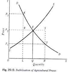
Consider figure 25.12 again.Suppose the government wants to stabilize prices at OP2 level.If the production for either year is OH, the government buys and stores QH quantities from the open market to keep the price at the level of OP2.

The farmer will give the full amount sold by OH, the OQ to the general public and the qh to the government.Thus, the income of the peasant will be OP2SH.On the other hand, if production for any of the years falls to the level of OL, in order to keep the price in OP2, the government will sell the amount of LQ from inventory on the open market.However, farmers sell only the amount of OL they produce,so the income they earn is equal to OP2RL.

This income earned by OP2RL will be much smaller than the OP ^ SH earned when production is OH.When the price is fixed at the level of OP2, farmers sell everything produced to the public and some to the government, so the income of the farmers changes as production changes.

Therefore, it is clear that the government can successfully stabilize prices through buffer inventory operations, but this price stabilization policy will not guarantee farmers a stable income.Indeed, at a price fixed by the government, the income of the peasants changes in direct proportion to the change in production, and a 10 percent increase in production leads to a 10 percent increase in the income of the peasants, and vice versa.

Therefore, government intervention in the above methods ensures price stability, but it does not exclude fluctuations in the income of farmers.Therefore, the purpose of price stability contradicts the purpose of income stability of farmers.

Income stabilization：

Now, the key question is what should the government do if it wants to stabilize the income of farmers.Stabilization of the income of peasants can be achieved by modestly changing prices.To stabilize the income of farmers, the government should allow changes in prices that are exactly proportional to unplanned changes in production.

In order to ensure income stability, if crop production increases by 10%, the government should only allow the fall in prices by 10%, and if crop production decreases by 10%, the government should only allow 10%.Rising prices.

Consider figure 25.13.Where DD is the demand curve for goods and SS is the planned production by farmers. 2 intersect at Point E.This indicates that the market price is OP and the planned equilibrium production is OQ.Let's assume that the actual unplanned production is different between OL and OH.

If this production variation is left free to affect the price, the market price will fluctuate between OR and OU.A single elastic demand curve D'd’(dotted line) passing through the point E was drawn to graph how much the price should be allowed to fluctuate in the face of actual production fluctuations in order to ensure the stability of farmers ’income.

It is reminded that in a single elastic demand curve, spending on goods by consumers remains constant.Thus, for each combination of price and quantity represented by this single resilient demand D'd’, the expenditure (and hence the income that the peasant earns) remains constant and is equal to the area of the rectangular OPEQ.

Now assume that the actual production for any given year is OH.If the market system is allowed to function freely, with the use of production OH, the price will fall to OR, and the income earned by the peasants will be equal to the area of the rectangular ORGH.From figure 25.13 it becomes clear that in production OH, the price should be allowed to fall from OP to OS level only if the income of OSJH (equal to the area of OPEQ) is guaranteed to the farmer.From figure 25.13, we can see that in the case of price OS, the government needs to buy the SZ quantity of the public purchase and the remaining quantity ZJ to keep the price in the OS.

On the other hand, when the actual output falls to OL, the market price rises to OU.However, in order to keep the income of farmers equal to the area of OPEQ or OSJH, prices need to be increased only to the OT level

If the production OL and the price are equal to OT, then the income of the farmer will be(97VL is equal to OPEQ or OSJH,and points V, E,and J are on a single elastic demand curve D'd'(dotted line)).At the price OT, consumers buy goods in TB quantity, and farmers production is only TV (=OL), so VB quantity, the government needs to sell to the public from the buffer stock.

If the above-mentioned income stabilization policy is carried out efficiently, the following benefits can be achieved.First, there is a gradual change in prices compared to too large changes in prices if left undetermined by the free market mechanism.

Secondly, even in the face of significant fluctuations in production, the income of farmers will stabilize at a certain level.Thirdly, the policy of income stabilization is self-financing, in fact, it can give the government a net profit.This is because the government buys at a lower price and sells at a higher price, as can be seen from figure 25.13.

Stabilization of peasant income by the government

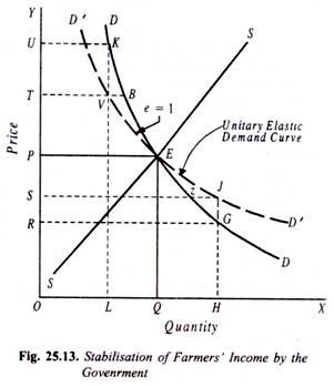
If the total profit is equal to the cost of storage of goods, then the scheme is fully self-funded.Therefore, whether there is a net profit or a net loss to the government from this scheme depends on the magnitude of the cost of storage.

This policy of income stabilization with gradual changes in prices is better than the policy of full price stabilization.Because in the case of a policy of full price stabilization, the government will buy and sell at the same price, so the cost of storage will not be met.

References

Https://opentextbc.ca/principlesofeconomics/chapter/8-1-perfect-competition-and-why-it-matters/

Https://www.economicsdiscussion.net/articles/short-run-and-long-run-supply-curves-explained-with-diagram/1677

Https://pressbooks.bccampus.ca/uvicecon103/chapter/4-4-elasticity-and-revenue/

Https://www.tutor2u.net/economics/reference/perfect-competition-assumptions-and-characteristics

Https://courses.lumenlearning.com/suny-microeconomics/chapter/efficiency-in-perfectly-competitive-markets-2/

Https://www.economicsdiscussion.net/monopoly/constructing-a-supply-curve-under-monopoly/17069

Principles of Microeconomics

Timothy Taylor, Saint Paul, Minnesota

Steven A. Green law, Fredericksburg, Virginia

Microeconomic theory Andreu Mas-Colell

Principles of Economics N. Gregory Mankiw