UNIT III
Production and Cost
Production function
To have clear knowledge about production and cost it’s mandatory to know the basics of production functions and understand the fundamentals in mathematical terms. We break down short-term and long-term production functions supported variable and glued factors.
What is the production function?
The functional relationship between the physical input (or factor of production) and therefore the output is named a production function. It assumed the input as an explanatory or independent variable and the output as a dependent variable. Mathematically, you can write this as:
Q=f(L,K)
Where"Q"represents the output,"L"and"K" are the inputs, respectively, labour and capital (such as machinery). Note that there may be many other factors, but we are assuming a two-factor input here. Production functions are defined differently in the short term and in the long term. This distinction is crucial in microeconomics. This distinction is based on the nature of the factor input.
Inputs that change directly with the output are called variable factors. These are factors that can change. Fluctuating factors exist both in the short term and in the long term. Examples of variable factors include daily labour and raw materials.
On the other hand, factors that cannot change or change as the output changes are called fixed factors. These factors are usually characteristic only for a short or short period of time. There are no fixed factors in the long term.
Therefore, two production functions can be defined: short-term and long-term. A short-term production function defines the connection between one variable factor (keeping all other factors fixed) and therefore the output. The law of regression to factors explains such a production function.
For example, suppose that a company has 20 units of Labour and 6 acres of land, and initially uses only Labour units (variable coefficients) for that land (fixed coefficients). Thus, the ratio of land and labour is 6: 1. Now, if the company chooses to adopt 2 labour units, then the ratio of land to Labour will be 3: 1 (6: 2).
Here, all factors change in the same proportion. The law used to explain this is called the law of return to scale. It measures how much of the output changes when the input changes proportionally.
Production requires the cooperation of certain factors. These are known as production agents. They are also called economic resources or inputs. Roughly, there are four agents: land, labour, capital and organization.
Production factors:
The production of goods or services requires the use of certain resources or production factors. They are called economic resources, because most of the resources needed to continue production are scarce compared to their demand.
Resources, which we call production factors, are combined by companies and companies in various ways, creating an annual flow of goods and services.
Each factor receives a reward based on its contribution to the production process, as shown in the table.
In fact, any community resource, called a factor of production, can be classified in different ways, but it facilitates the generally acceptable classification, keeping in mind that the production of goods and services is the result of people working in natural resources and equipment such as tools, machinery and buildings. There is a time separated from the rest of the company, which is the fourth factor that distinguishes the company from the rest.
People involved in production use their skills and efforts to create things and do what is desired. This human effort is known as Labour. In other words, labour represents all human resources. The natural resources that people use are called land. And the equipment they use is called capital, and this refers to all artificial resource
(1) Land and Natural Resources: In economics, the term land, in a broad sense, is used to refer to all natural resources or gifts of nature. As the Penguin Dictionary of Economics puts it:"the land of economics is taken to mean not just a part of the Earth's surface covered with water, but also all the free gifts of nature, such as minerals, soil fertility, and also the resources of the sea. Land provides both space and specific resources".
From the above definition, it is clear that the land includes agricultural and architectural lands, forests and mineral deposits. All those natural resources (or gifts of nature) that help us (members of society) to produce useful goods and services such as fishing, rivers, lakes. In other words, the land contains not only the surface of the land, but also sea fish, the sun's heat, which helps to dry the grapes and turn them into resin, rain, which helps farmers grow their crops, the Earth's surface.
The first three factors—land; labour and capital do not work independently or in isolation. It is necessary to combine these factors and adjust their activities. These two functions are performed by the organizer or entrepreneur.
Features:
The land has certain important properties:
1. Fixed supply: The total land area of the Earth (in the sense of the surface area available to men) is fixed. Therefore, the supply of land is strictly limited. It is definitely possible to increase the supply of land in a particular area to some extent through land reclamation and deforestation from the sea area. However, this is often offset by various types of soil erosion. The end result is that the change in the total area does not really matter. Of course, the effective supply of agricultural (farm) land can be increased by the use of drainage, irrigation and Fertilizers.
As a result, the price of land and natural resources becomes very sensitive to changes in consumer demand and tends to rise sharply when it becomes more desirable. In this context, we can see a sharp increase in the price of Bombay building land in the last fifty years. But new discoveries are often stimulated by higher prices (as is the case in the Salt Lake region of Calcutta), and like oil in the UK's North Sea, prices tend to rise modestly.
2. Alternative use: The total supply of land is fixed, but the land has alternative uses. The same plot of land can be used to establish factories, grow wheat and sugar cane, and build stadiums. This means that the supply of land to a particular application is quite (if not complete) elastic. For example, the amount of land used for growing tomatoes can be increased by reducing the cultivation of other crops (for example, cauliflower). The supply of building land can be increased by reducing the area under agricultural operations.
3. No production cost: Since land is a gift of nature, there is no cost of production. Since the land already exists, there will be no costs when creating it. In this sense, the land is different from both labour (it must be nurtured, educated and trained) and capital (it must be created by using labour and other scarce resources or spending money).
Thus, logically, the entire return from the land—called rent-would be (at least from the point of view of society) surplus income. As Stanlake rightly puts it, “an increase in the value of natural resources due to population growth and income growth will result as a windfall benefit to the owners of these resources."
However, the above argument is not valid today. In fact, many of the Land Services require the expenditure of resources to acquire or maintain them, and therefore land as a factor of production they are often referred to as capital (i.e. means of production) is something “really different “from capital.
But this is not the only feature of entrepreneurs. The decision to produce something must be taken in anticipation of demand, and there must be an element of uncertainty about what that demand will materialize.
Therefore, risk-taking or companies can be considered as the fourth factor in production, and those responsible for taking these risks are usually referred to as entrepreneurs (see box below which is self-evident). Against this background, one can study the properties and properties of the four factors. But before we go further, we can make a passing reference to factor mobility.
4. Fertility differences:
Another important feature of the land is that it is not homogeneous. All grades of land (plots) are not equally productive or fertile.. And Ricardo argued that the rent was caused not only by lack of land as a factor, but also by differences in soil fertility.
5. Operating the law to reduce returns:
Finally, we can refer to the special features of the land that are not shared by other factors. In fact, land production is subject to the operation of the law of reduction return.
This simply means that as more workers are employed on the same parcel of land, the output per worker gradually decreases (as each additional worker contributes less to the total product contribution). The law of reducing returns refers to reducing the marginal product of variable factors.
- Mobility:
The land is not geographically mobile. But it is professionally mobile. For example, in most parts of India, land has many alternative uses. For example, some of the hilly lands such as Shilong and Darjeeling have extremely limited occupational mobility as they are useful as sheep grazing, golf courses or tourist centres.
- Return:
The income received by the owner of the land is known as rent. It can be noted that the rent is usually paid for more than the use of land and other natural resources, but it is necessary to make the resource available in a usable form.
An example of this is labour that helps in the process of bringing minerals to the surface. While it is still under the ground, iron ore is useless. It can increase the productivity and value of the land if it is improved by fertilizer, irrigation, construction of fences and buildings. So the rent paid for this kind of fertile land is rather a mixed type of factor income.
(2) Labour:
Like land, labour is also the main factor in production. A feature of the factor of production, called labour, is that it provides Human Services. It refers to all kinds of human influences, physical and mental, which are directed at the production of goods and services. "Labour" is a collective term given to productive services embodied in human physical exertion, skills, intellectual abilities, etc.
So, there are different types of labour inputs, which differ in the content of efforts and skills, especially in the content of skills. Therefore, as in the “land", labour is not homogeneous. The term covers clerical, administrative and administrative functions, as well as skilled and unskilled manual work.
Land and labour:
Labour differs from land in a significant way. Land is a stock, but Labour is a flow. The term “labour" is used to refer to the flow of labour services per unit of time. So labour is perishable. If we don't take advantage of today's workforce, a large amount will not be available tomorrow (and in the future) accordingly.
In this context, it is necessary to note relevant but important points. In other words, it is not labour itself that is bought and sold, but the services of Labour. Companies cannot buy and sell labour in the same way they can buy land or capital.
Dual role:
Another important point is that Labour is not a factor. Workers-workers ' suppliers are also consumers. Thus, labour plays a dual role in the modern economy. Labour is the subject of production, and also the object of production.
This means two things.
(1) The use of Labour is necessary for the production of something.
(2) Almost everything is produced to meet the needs of the main consumer workers. In fact, any economic activity is carried out to satisfy consumers. The businesses of consumption demand, and produce incentives.
Peculiarities of labour as a factor:
When examining the labour market, it is important to realize that Labour has many special features that distinguish it from ordinary goods.
1. First, trade in the labour market is particularly important.
First, labour market transactions are especially important for individual workers. Much of a person's lifestyle and relationships with others depends on the work he or she does. In addition, the employment of labour involves a continuous personal relationship between the employer and the employee, while the trade in the market of goods is often concise and inhuman.
Production function
To have clear knowledge about production and cost it’s mandatory to know the basics of production functions and understand the fundamentals in mathematical terms. We break down short-term and long-term production functions supported variable and glued factors.
What is the production function?
The functional relationship between the physical input (or factor of production) and therefore the output is named a production function. It assumed the input as an explanatory or independent variable and the output as a dependent variable. Mathematically, you can write this as:
Q=f(L,K)
Where"Q"represents the output,"L"and"K" are the inputs, respectively, labour and capital (such as machinery). Note that there may be many other factors, but we are assuming a two-factor input here. Production functions are defined differently in the short term and in the long term. This distinction is crucial in microeconomics. This distinction is based on the nature of the factor input.
Inputs that change directly with the output are called variable factors. These are factors that can change. Fluctuating factors exist both in the short term and in the long term. Examples of variable factors include daily labour and raw materials.
On the other hand, factors that cannot change or change as the output changes are called fixed factors. These factors are usually characteristic only for a short or short period of time. There are no fixed factors in the long term.
Therefore, two production functions can be defined: short-term and long-term. A short-term production function defines the connection between one variable factor (keeping all other factors fixed) and therefore the output. The law of regression to factors explains such a production function.
For example, suppose that a company has 20 units of Labour and 6 acres of land, and initially uses only Labour units (variable coefficients) for that land (fixed coefficients). Thus, the ratio of land and labour is 6: 1. Now, if the company chooses to adopt 2 labour units, then the ratio of land to Labour will be 3: 1 (6: 2).
Here, all factors change in the same proportion. The law used to explain this is called the law of return to scale. It measures how much of the output changes when the input changes proportionally.
The law of variable proportions or the return to factors plays an important role in the study of the theory of production. In this article, we will look at the meanings, explanations, stages, significance, and reasons behind the operation of the law of variable proportions.
Law of variable proportions or factor of a variable
This law indicates a short-term production function in which one factor changes and the other is fixed.
Also, if you get an extra output when applying an extra unit of input, this output will be equal to or less than the output obtained from the previous unit.
The law of variable proportions relates to how the output changes when the number of units of variable factors is increased. Thus, it refers to the effect of the changing factor ratio on the output.
In other words, this law shows the relationship between the unit of variable factors and the volume of production in the short term. This assumes that all other factors are constant. This relationship is also known as the return to variable factors.
The law states that if we keep other factors constant, then when we increase the variable factor, the total product first increases at the rate of increase, then at the rate of decrease, and finally begins to decrease. Why is it called the law of variable proportions?
The factor ratio or factor ratio changes because one input changes and everything else remains constant. Let's take an example to better understand this:
Let's say you have 10 acres of land and 1 unit of labour for production. So, the ratio of land and labour is 10: 1. Now, if we increase the unit of Labour to 2 while keeping the land constant, then the ratio of land to Labour will be 5: 1.
Thus, as you can see, the law analyses the effect of changes in the factor ratio on the amount of out, and hence is called the law of variable proportions.
The law of proportion of variables explained
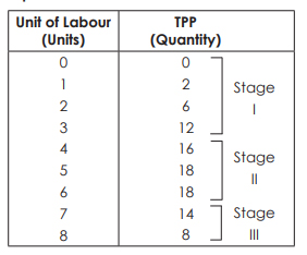
Let's understand this law with the help of another example:
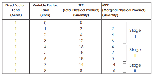
In this example, land is a fixed factor and labour is a variable factor.
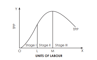
The following figure describes the law of variable proportions. For a simple representation, the total physical product (TPP) curve and the limit physical product (MPP) curve are drawn as smooth curves for variable inputs (labour).Three stages of law
The law has three stages:
Stage I–TPP will increase at an increasing rate, and MPP will increase too. The MPP increases with the increase of the variable factor unit. Therefore, it's also called the stage of accelerating returns. In this example, Phase I of the law runs up to three units of labour (between points O and L).
Stage II–TPP continues to increase, but is declining. But the increase is a plus. In addition, the MPP decreases with an increase in the number of units of the variable factor. Therefore, it is called the stage of Return of decline. In this example, Stage II is performed between four to six units of labour (between points L and M). This stage reaches the point where TPP is maximum (18 in the example above) and MPP is zero (point R).
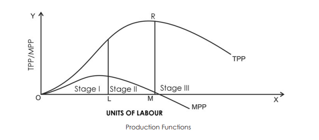
Stage III- now the TPP begins to decrease, the MPP decreases and goes to the negative. Therefore, it's called the stage of negative returns. In this example, Stage III is performed between seven and eight units of labour (from Point M onwards).
Significance of three stages
Stage I
At this stage, the marginal product increases with an increase in the variable factor.
Thus, producers can adopt more units of variables to efficiently utilize fixed factors. So the producers would prefer not to stop at stage I, but try to expand further.
Stage II
Producers do not like to work even in Stage III. At this stage, there is a decrease in the total product, and the marginal product becomes negative.
To increase output, producers reduce the amount of variable factors. However, in Stage III, the cost of generating an increase will be less profitable and the profit will decrease.
Stage III
Any intelligent producer avoids the first as well as the third stage of production. Therefore, producers prefer Stage II–a stage that reduces returns. This stage is the most relevant stage of operation for producers, according to the law of variable proportions.
The law of variable proportions in terms of TPP and MPP
The description is as follows:
The law of the rate of change-from the perspective of the TPP
We know that the law of variable proportions shows the relationship between the units of variable factors and the total physical product.
Also, if you keep other factors constant and increase the unit of variable factors, the TPP will initially increase at the rate of increase, then decrease, and eventually decrease. So there are three distinct stages:
I-TPP is increasing at an increasing rate
II-TPP is increasing at a declining rate
III-TPP decline
Example of the law of variable ratios from the point of view of MPP and from the point of view of TPP Law
I-MPP increase
II-MPP decreases, but remains positive
III-MPP continues to decrease and becomes negative
Reasons for the operation of the law
In the short term, we cannot change all the factors of production.
In this case, there is only one variable factor, and the other is fixed.
All other factors combine optimally to produce maximum output.
Thus, the marginal physical product increases.
In the early stages, when producers adopt more units of variable factor versus fixed factor, the total product tends to rise at an increasing rate.
Then, beyond the point of optimal combination, if the producer adopts more units of variable factors, the factor proportion becomes inefficient. Thus, the marginal product of its variable factor decreases.
Also, producers see that as they increase the unit of variable factors, the amount of fixed factor input per unit of variable decreases.
Therefore, successive units of variable inputs add the reduced amount to the total output because there are fewer fixed inputs to operate.
In this article we will discuss the company's isoquant under return to scale.
It is assumed that the amount of all inputs used by the enterprise will change by the same percentage. So if a company uses only two inputs, X and Y, these inputs will always be used at a certain percentage.
For example, in Figure 8.22, if you use a particular input combination a (x1, Y1) on any straight line through the origin, such as OE, the ratio of y to X Y1/x1 is itself the slope of the line OE.
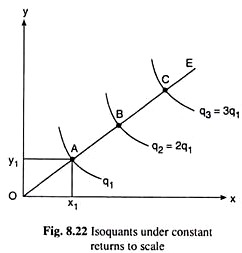
If you plan to use another combination of inputs by changing X and y at the same ratio, i.e. with a fixed input percentage, you need to move to another combination along the oe line. Because at any (x, y) Point on the line OE, the slope or y/x ratio of the line is known to be constant.
Also, from simple mathematics, if a company moves from any point A to another point B along a straight line OE, the proportional change in x and y is the same as the ratio of distance OB to distance OA, for example, in the diagram. 8.22, if OB=2.The OA would say, compared to point A, the company's use of both inputs has doubled at Point B.
Here, if the output at point A is q=q1, then for a constant return to the scale, at Point B, q=2q1=q2 (for example), where the output along the equivalent through a is q=q), and the output along the equivalent through b is q=q2 = 2q1.
Similarly, if the company moves from point B to Point C along the straight line OE, and there is AB=BC or OC=3.0 A, then compared to point A, x and y at Point C will be three degrees, and for constant returns, the output at C, or Q=3q1=q3 from IQ along C (for example).
Therefore, that in the figure. 8.22, if the constant returns to the scale, moving along a straight line (or ray) like oe, the origin (O) and IQ, q1, IQ, q1 and IQ, 2q1, IQ, 2q1, IQ, 3q1,...We can see that the distances between (BC) are all equal to each other (OA=AB=BC).=..................).
That is, the IQ map is shown in the figure. 8.22 represent the constant return on the scale.
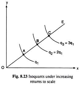
IQ map in the figure. On the other hand, 8.23 represents the law that increases the return to the scale. Here, along the Ray OE, oa>AB>BC>...Points A, B, C,...The output is on q1, 2q1,3q1,IQs. . . . Since AB<OA here, OB<2OA, i.e. while moving from point A to point B, the company increased x and y to less than double, but the output doubled from q1 to 2q1.
That is, in this case, the output is increasing more than in proportion to the increase in the amount of input. Thus, the return to scale is increasing. Similarly, if BC<AB, etc. We would also get an increasing return on the scale.
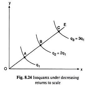
Finally, the IQ map is shown in the figure. 8.24 represents the law of reduction of return to scale. Here along the oe line, point A, B, C,OA<AB<BC<...There are many ways to do this. . . Output q1, 2q1,3q1,...Here, AB>OA,so OB>2.While moving from point A to point B along OA, i.e. oe, the company doubled the amount of input X and Y,and the output doubled from q to 2q.
That is, in this case, the output is increasing less in proportion to the increase in the amount of input. Thus, the return to scale has decreased. Similarly, if BC>AB, etc. It also gives a reduction to scale.
Economies of scale are defined as cost advantages that an organization can achieve by expanding its production over the long term.
In other words, these are the benefits of large-scale production of the organization. Cost benefits are achieved in the form of a low average cost per unit.
It's a long-term concept. Economies of scale are achieved when the turnover of the organization increases. As a result, the savings of the organization will increase, and it will be even more possible for the organization to obtain large amounts of raw materials. This will help the organization to enjoy discounts. These benefits are called economies of scale.
Economies of scale are divided into internal and external economies, which are discussed as follows:
i.Internal economy:
See the real economy arising from the expansion of the plant size of the organization. These economies arise from the expansion of the organization itself.
An example of an economy of internal size is:
a.Technical economy of scale:
It occurs when an organization invests in expensive and advanced technologies. This helps to reduce and control the production costs of the organization. These economies are enjoyed due to the technical efficiency obtained by the organization. Advanced technology allows organizations to produce a large number of goods in a short time. Thus, the industry-wide economy falls per unit of production costs
b.Marketing economy of scale:
Scale marketing economy is achieved in case of bulk purchase, branding, and advertising when large organizations have broadened their marketing budgets over large output. For example, large organizations enjoy the benefits of advertising costs as they cover a larger audience. On the other hand, small organizations pay the same advertising costs as big ones, but do not enjoy such benefits in advertising costs.
c.Financial economy of scale:
This happens when large organizations borrow money at a lower rate of interest. These organizations have good credibility in the market. In general, banks prefer to grant loans to organizations that have a strong foothold in the market and have good repayment capacity.
d.Management economy of scale:
During the occurrence of large organizations specialized workers for different things. These workers are experts in their respective fields and use their knowledge and experience to maximize the benefits of the organization. For example, in an organization, accounts and research departments are created and managed by experienced individuals so that all costs and benefits of the organization can be properly estimated.
E.Commercial economy:
See an economy where organizations enjoy the benefits of purchasing raw materials and selling finished products at a lower cost. Large organizations buy raw materials in bulk; therefore, enjoy the advantages of transportation charge from Bank, easy credit, and prompt delivery of products to customers.
Ii.Foreign economy:
Occurs outside the organization. These economies arise within industries that benefit organizations. If the industry expands, the organization will benefit from better transport networks,infrastructure and other facilities. This will help reduce the cost of the organization.
Some examples of economies of external scale are discussed as follows:
A.Economy of concentration:
See the economy resulting from skilled labor, better credit, and the availability of transport facilities.
B.Economy of information:
Means the benefits gained from trade and business related publications. The central research institution is the source of information for the organization.
C.Collapsing economy:
Refer to the division of associations caused by the economic process into different processes.
Uneconomics of scale occurs when the long-term average cost of an organization increases. It can occur when the tissue becomes excessively large. In other words, uneconomics of Scale Causes larger org-anizations to produce goods and services at increased costs.
There are two types of scale diseconomies: internal diseconomies and external diseconomies, which are discussed as follows:
i.Internal uneconomics of the scale:
See uneconomical raising the cost of production in the organization. The main factors affecting the cost of production of the organization include the lack of determination, supervision and technical difficulties.
Ii.External uneconomics of the scale:
See uneconomical to limit the expansion of an organization or industry. Factors acting as restraints on expansion include increased production costs, a shortage of raw materials and a decline in the supply of skilled workers.
There are several causes of diseconomics of scale.
Some of the causes that lead to uneconomics of scale are:
i.Act as the main reason for diseconomics of scale.
If the organization's production goals and objectives are not properly communicated to employees in the organization, they can lead to overproduction or production. This can lead to diseconomics of scale.
Separately, if the communication process in the organization is not strong, then the employee will not get enough feedback. As a result, there will be less face-to-face interaction between employees, which will affect the production process.
Ii.Lack of motivation:
This leads to a decrease in productivity levels. For large organizations, workers may feel isolated and less motivated because they are less valued for their work. Because of poor communication networks, it is difficult for employers to interact with employees and build a sense of attributes. This leads to a decrease in the productivity level of output due to lack of motivation. This further leads to an increase in the cost of the organization.
Iii.Loss of control:
It serves as the main problem of large organizations. Monitoring and controlling the work of all employees in a large organization becomes impossible and expensive. It is difficult to make sure that all employees of the organization are working towards the same goal. It becomes difficult for managers to direct the sub-coordinates of large organizations.
Iv.Cannibalism:
It means a situation where an organization is facing competition from its products. While smaller organizations face competition from the products of other organizations, larger organizations find their products compete with each other.
Cost behavior in the short term
Short-term costs are important for understanding costs in economics. Short-term and long-term distinctions based on fixed and variable factors of production make the concept of understanding short-term costs easier. Let us understand the concept using examples, diagrams for graphical representation.
Short run concept
To understand short-term costs, it is important to understand the concept of short-term costs. In economics, we distinguish between short-term and long-term through the application of fixed or variable inputs.
Fixed input (plant, machine, etc.)) is a factor of production that can not be changed or changed in a short span because the period is"too small". This will be short-term. Here, the inputs are two types: fixed and variable.
In the long run, all inputs will be mutable(e.g.. Raw materials). This means that all inputs can be changed as the output volume changes. Therefore, the concept of fixed input applies only in the short term. It is in the short-term cost that we turn this time.
It explains that the cost of production depends on the level of output, given that others remain the same (ceteris paribus). This can be mathematically written as:
C=f(X)
Where C is the production cost and X is the output level.
Total fixed costs
Fixed cost refers to the cost of fixed input. At the level of output it does not change (hence, fixed). Fixed inputs include buildings,machines, etc. Thus, the cost of inputs, such as rent and the cost of machines, constitute a fixed cost. Also known as overhead, supplemental or overhead, these costs remain the same regardless of the level of output.
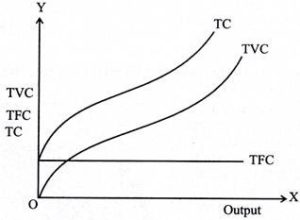
So if you plot the total fixed cost (TFC) curve against the output level on the horizontal axis, you get a straight line parallel to the horizontal axis. This indicates that these costs remain the same and should occur even if the output level is zero.
Total variable costs
The costs incurred by variable factors in production are called Total variable costs(TVC). These costs differ in the level of output. Therefore, when the production level is zero, the TVC is also zero. Thus, the TVC curve begins at the origin.
The Shape of the TVC is unique. It is said that it has the form of an inverted S. This is because, in the early stages of production, there is a scope for efficient use of fixed factors by using more variable factors (e.g., variable factors). Workers who use the machine).
Thus, as the variable input used increases, the production efficiency of the variable input ensures at a rate at which the TVC increases but decreases. This makes the first part of the tvc curve concave.
As production continues to increase, more variable factors are employed for a given amount of fixed inputs. The production efficiency of each variable factor is reduced,adding more to the production cost. Therefore, TVC will increase,but now it is increasing at the rate of increase. This is where the shape of the TVC curve is convex. Thus, the TVC curve will have an inverted-S shape.
Total cost
Total cost(TC) refers to the sum of fixed and variable costs incurred in the short term. So, the short-term cost can be expressed as follows
TC=TFC+TVC
Note that in the long run, TFC=0, so TC = TVC. So you can get the shape of the TC curve by summing the TFC curve and the TVC curve.
For the TC curve, the following points can be noted:
- The TC curve is shaped of reverse S. This is because of the TVC curve. Since the TFC curve is horizontal, the difference between the TC curve and the TVC curve is the same at each level of the output and is equal to the tfc. This is explained as follows: TC-TVC=TFC
- The TFC curve is parallel to the horizontal axis, and the TVC curve is inverted S-shaped.
- The law that explains the Shape of TVC and subsequent TC is called the law of variable proportions.
Maximize profit and minimize costs
The problem with Rm is to maximize the pro ts by selecting the optimal amount. Adopt to generate input and output of. We already know how to solveproblem of Profit Maximization issues in a competitive market environment. This direct approach shows the sights of some tourism. There are some very important insights, especially on the cost side of the rm problem, such as You can get it if you look at rm problems through a more indirect approach. The idea is rm Pro t maximize problem to break down into two stages: RST, we look the problem of minimizing the cost of producing any given amount of output, and secondly, we look these notes cover the first of these two stages, namely they answer the question: for given the amount of output, y (just some number, 10, 20, 100, this is not always necessary what is the minimum cost of production (that the optimal output of rm will result in it producing that's it. In other words, given that you need to generate the output and y units of the given input. Price W1 and W2, rm how much each input should be employed to generate y at minimum a costly way. Note that the amount of each input used depends on the output if you want to generate an output of the level-1000 units that rm wants to generate, it would be definitely need more workers and machines than just producing 10 units. Keep in mind that cost minimization is a requirement for competitive Profit maximization Market. If you do not minimize the cost for a given level of output, it means that he is also Profit is not maximization. Why? Since the revenue of a given Y is Xed (taking p as given), if there is a to generate this output level.
Difference between conditional input requests from cost minimization problem and (unconditional) input request from Profit maximized problem .It is important to understand that this comes from a conditional input request. The above cost minimization problem is not the same as (unconditional, sometimes input requests resulting from pro t maximization problems(See note above)
Profit maximization and input request). Remember the Profit to maximize input requests,
(W1; W2; P) was a function of input price, W1 and W2 and output Price p:they are called unconditional(or simply not conditional) depending on Y-rm's Pro t maximize problem output level is already optimized. And this optimized output level would be a function of price (W1;W2;p), given by the following formula-so the (unconditional) input request is just a function of the given one, i.e. the given one price. In contrast, the cost minimization problem is solved for a given output level it's not always the optimized one that rm ultimately chooses. The problem of cost minimization was only the first step in an indirect approach to solve.
With the problem and its first step, the output level was taken as given. How to produce a certain output level at minimum cost. Therefore, the request for conditional input. It only depends on what is given in the cost minimization problem, i.e. input price, W1 and W2. And the output level Y: again: the (unconditional) input request depends on the output Price, P, conditional input request depends on output level and Y: both of them Input price, W1 and W2.
The enterprise is in equilibrium when there is no desire to change (increase or decrease) its output level. At the equilibrium point, the company earns the maximum profit. In this article, we will discuss two approaches to the equilibrium of the enterprise and the equilibrium of the producer.
Company objectives
The main objectives of the company are:
Achieve the target rate of return
Stabilize price and profit margins
Achieving target market share
Prevent price competition
Maximize sales or sales revenue
For a really while people believed that the only purpose of the corporate is to maximise profits. After all, every business wants to earn the maximum profit,right? But over the years beliefs have changed. Now it is believed that the only purpose is the maximization of profits only in the case of a single owner company.
Producer's equilibrium
The producer's equilibrium is the level of production of goods that gives the maximum benefit to the producer of goods. If there is no scope for reducing losses by increasing profit revenues or changing output quality, companies are in equilibrium. Therefore, we
Profit (△)=total revenue–total cost=TR-TC
Thus, the output level at which the output level minus the total cost from the total revenue is the maximum is the equilibrium level of the output. There are two approaches to reaching a producer's equilibrium:
Total revenue-total cost (TR-TC) approach
Marginal revenue-marginal cost (Mr-Mc) approach
Here you will learn the basic concepts of earnings.
TR-TC approach
According to this approach, the equilibrium of producers has two conditions:
- The difference between TR and TC is that the largest
- Even if one more output unit is generated, the profit will fall. In other words, when another unit is produced, the marginal cost will be higher than the marginal revenue.
In today's times, the manager's salary and benefits are related to turnover (not profit). Even financial institutions easily provide credit to companies with increased turnover. .
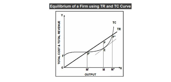
In in the figure above, the X-axis shows the level of output, and the Y-axis shows the total cost and total revenue. TC is the total cost curve and TR is the total revenue curve. Also, P is the equilibrium point at which the distance between TR and TC is greatest.
In addition, we can see that there is TC>TR before the point P'and after the point P". Therefore, producers must produce between P'p"or M'm". At the point P, The Tangent drawn to TC is parallel to TR. In other words, at the point P, the slope of TC is equal to the slope of TR.
Mr-Mc approach
The Mr-Mc approach springs from the TR-TC approach. The two provisions of equilibrium under the Mr-Mc approach are:
MR=MC
MC cuts the Mr curve from the bottom
MR=MC
If one additional unit of output is generated, MR is the gain and MC is the cost to the producer. As long as MR is larger than MC, it is beneficial to produce more. Therefore, the company has not achieved an equilibrium level of output, where the profit is maximum. This is due to the increase in profits at the Enterprise manufacturing.
On the other hand, if MR is less than MC, the profit will be less than the cost. Therefore, producers are also not in equilibrium. He can reduce production to add to his profits. If MC=MR, then the profit is equal to the cost,and if MC exceeds this level of output and is greater than MR, then the producer is in equilibrium.
Therefore, for the equilibrium of producers, MC=MR is a necessary condition, but not sufficient. Here we will understand in detail the equilibrium in Monopoly.
MC cuts the Mr curve from the bottom
MC=MR is necessary for equilibrium, but that is not enough. This is because the producer may face multiple MC=MR outputs. Of these, only those outputs where MC is greater than MR are balanced outputs.
This is because if MC is greater than MR, then producing above MR=MC will reduce the profit. Also, when you can no longer add profit, you will reach the maximum profit level.
On the other hand, if the MC exceeds the MC=MR output and is smaller than MR, the producer can add a profit by producing more. Therefore, for the equilibrium of producers, MC=MR.It is also important that the MC must be greater than the MR if more output is to be produced.

Very long-term production differs from long-term production in that there may be technological changes. There are three main types of technological advances:
New technologies allow for completely new products
- The new technology allows us to produce equal quantities with less input, replacing our isoquants.
- New technology enables us to produce more with equal input, replacing our production function
- These technological advances can replace the ratio of capital and labor in one or the other way. Let's first look at it graphically

The first technological change, shown in the adjacent diagram, is called Hicks-neutral, which translates into an invariable ratio of the marginal product of capital and the marginal product of Labor. John Hicks invented it in his book"The Theory of wages", 1932. Analytically: Y = AF (K, L))
- The second technological change is called Harrod neutral or labor augmentation to improve the efficiency of Labor. Roy Harrod formulated it in his 1948 book toward dynamic economics. Analytically: Y=F(K, AL)
- The third and last technological change shown is named Solow-neutral or capital-augmenting, which increases the efficiency of capital. This was devised by Robert Thoreau in his article"technological changes and aggregate production functions"in 1957. Analytically: Y=F(AK, L)
Finally, we must also take into account the potential for endogenous growth resulting from endogenous technological changes. This can be easily plotted by using the Cobb-Douglas function like this:

References
Https://opentextbc.ca/principlesofeconomics/chapter/8-1-perfect-competition-and-why-it-matters/
Https://www.economicsdiscussion.net/articles/short-run-and-long-run-supply-curves-explained-with-diagram/1677
Https://pressbooks.bccampus.ca/uvicecon103/chapter/4-4-elasticity-and-revenue/
Https://www.tutor2u.net/economics/reference/perfect-competition-assumptions-and-characteristics
Https://courses.lumenlearning.com/suny-microeconomics/chapter/efficiency-in-perfectly-competitive-markets-2/
Https://www.economicsdiscussion.net/monopoly/constructing-a-supply-curve-under-monopoly/17069
Principles of Microeconomics
Timothy Taylor, Saint Paul, Minnesota
Steven A. Green law, Fredericksburg, Virginia
Microeconomic theory Andreu Mas-Colell
Principles of Economics N. Gregory Mankiw