UNIT IV
Market Structure
Perfect competition refers to a market situation in which there are a large number of buyers and sellers of homogeneous products.
The price of a product is determined by the industry by the forces of supply and demand. For example, if you need a pen, there should be several shops selling pens. Under the conditions of perfect competition, every seller must sell the same quality of the pen at a uniform prevailing price on the market. You can buy a pen from any store at the price Rs. 10. If another shopkeeper charged Rs. 12 for the same quality of the pen, nobody buys from him. But if the shopkeeper charged Rs. 9 all buy pens from that particular store. But both of these situations are unrealistic.
There must be one price dominant throughout the market. Therefore, full competition in the market structure is characterized by a complete lack of competition between individual companies.
Definition:
It is identified by the existence of the many firm; they all sell an identical products an equivalent way. The supplier is the one who accepts the price."- Vilas
Such market gains when the request for product of every producer is totally elastic. Mrs Joan Robinson.
It is a market condition with an outsized number of sellers and buyers, similar products, free entry of enterprises into the industry is ideal knowledge between buyers and sellers of existing market conditions and free mobility of production factors between alternative uses. Lim Chong-ya
Assumption:
The following assumptions for a fully competitive market:
1. A large number of buyers and sellers:
This affects single buyers and sales. When a company enters or leaves the market, there is no impact on the supply. Similarly, if a buyer enters or withdraws from the market, demand will not be affected. Such affects individual buyers and sellers.
2. Homogeneous products:
The second assumption of perfect competition is that all sellers sell homogeneous products. In this situation, the buyer has no reason to prefer the product of one seller to another. This condition exists only if the goods have a clear chemical and physical composition, that is, Substances of the specified grade: salt, tin, wheat, etc.
3. No discrimination:
Under complete competition in the market, sellers and buyers, sellers do freely. It means that buyers and sellers must be willing to deal openly with each other to buy and sell at market prices. This may be true of everything you might want to do so without offering special deals, discounts, or favours to selected individuals.
4. Perfect knowledge:
The competitive market is me (buyers and sellers are in close contact with each other. It means that, on the part of buyers and sellers, there is complete knowledge of the market. This means that many buyers and sellers in the market know exactly how much the price of the goods is in different parts of the market.
In other words, there is full knowledge of each buyer and seller of the price at which the transaction is taking place, and the price at which the other buyer and seller are willing to buy or sell.
5. Industry FREE entry and exit:
In the long run, under full competition, the company can enter or exit the enterprise. There is no let or hindrance to the enterprise with regard to its entry into or exit from the market. In other words, the company has no legal or social restrictions. A large number of sellers is possible only if there is a free entry of the enterprise.
6. Perfect mobility:
There must be full mobility of domestic production factors that ensure uniform production costs throughout the economy. That means you are free to seek employment in any industry where different factors in production might like you.
7. Profit maximization:
Under perfect competition, all companies have a common goal of maximizing profits. Thus, there is a lack of social welfare of the general public.
8. No sales cost:
Under perfect competition, there is no sales cost.
9. No transportation costs:
Transportation costs between the sellers should not be. If transportation costs are present buyers are prevented from moving from one seller to another to take advantage of the price difference, which means that transportation costs do not affect the pricing of the product. In other words, these are always prices uniform in the market.
Pure and perfect competition:
Many economists choose to use the term "free market" rather than" pure competition.", American economists particularly prefer the term pure competition over the term perfect competition, but the term perfect competition seems to be popular with British economists.
But Professor Chamberlain distinguished between perfect competition and pure competition. Contains pure competition, according to Professor Chamberlain:
(I) numerous buyers and sellers,
(II) Homogeneous products,
(III) Free entry and exit of industry,
(IV) free from checks,
(V) lack of sales costs, and
(VI) lack of transportation costs.
R. A. Professor Bilas also distinguished between perfect competition and pure competition “perfect competition means pure competition, but we also consider other characteristics. Pure competition implies a certain degree of perfection, that is, the complete absence of monopoly.
In general, perfect competition leads to perfect resource mobility and perfect knowledge concepts. Similarly, professor Baumol defined pure competition as industry. Many companies are said to operate under pure competition when there is, product homogeneity, freedom of entry and exit, independent decision making.”
Based on these definitions, we can say that pure competition exists when an element of Monopoly is not present in the market. Perfect competition is wider than pure competition, including the absence of monopolies, as well as perfection in many other ways, such as full mobility of production factors and full knowledge of the market. Therefore, producers have complete knowledge of the quantity and quality of available production factors, as well as the prices that can be charged for their products.
Therefore, the distinction between pure competition and perfect competition is simply of a degree, and all assumptions of pure competition are also assumptions of perfect competition the concept of a complete competition system includes one more assumption: viz.Be perfect knowledge by both buyers and sellers of prevailing market prices, and different range and quality of various goods, services and production factors.
From the market demand curve, it's possible to derive the entire expenditure of the buyer, which forms the entire income of the enterprise that sells a specific commodity.
The total revenue is the product of the quantity sold and the price, and if the market demand is linear, the total revenue curve will be a curve that first tilts upwards, reaches the maximum point, and then begins to decrease (figure 2.40). For example, in Figure 2.39, the entire revenue at price P2 is that the area of the rectangle P2AQ20.
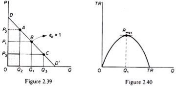
Of particular interest to the theory of the company is the concept of marginal income. Marginal revenue is a change in the total revenue that occurs as a result of selling additional units of goods.
Graphically marginal revenue is the slope of the total revenue curve at any level of output. If the demand curve is linear, it is clear that in order to sell an additional unit of x, its price must go down.
Since the entire quantity are going to be sold at a replacement low price, the marginal revenue are going to be adequate to the worth of the additional unit sold minus the loss from selling all previous units at a new low price somewhere qn is the quantity sold before the price falls.
MR = Pn+1 – (Pn – Pn+1) Qn
Obviously for all prices, MR is less than the price if (Pn–Pn+1) (=ΔP) is positive and Qn is positive.
Graphically marginal revenue can be derived from the demand curve as follows: Select any point of the demand curve (such as Point A) and from there draw perpendicular lines on the price and quantity axes (AP and AQ, respectively). Then find the midpoint of the vertical PA.
In Figure 2.41, the midpoint of PA is C draw a straight line from D to C and extend the vertical AQ until you cut it (at Point B in Figure 2.41). This line is the marginal earnings curve. To see it, we first note that the entire income in price P (=OPAQ) is that the sum of the marginal income of all individual units (=ODBQ) two areas, OPAQ, and ODBQ are actually equal; since they have a common area OPCBQ, and the Triangle DPC and CAB are equal (they have a corresponding angle equal). One side is equal by construction PC=CA).
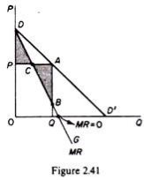
Thus, the MR curve is a line DCBG, which can be derived by coupling the midpoint of the perpendicular drawn from the demand curve to the price axis. In other words, the MR curve cuts such a vertical at its midpoint (if the demand is a straight line).
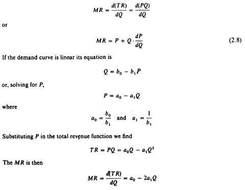
This proves that the MR curve starts at the same point (a0) as the demand curve, and that MR is a straight line with a negative slope that is twice as steep as the demand curve slope. This is the same result we established above using simple geometry.
The relationship between marginal income and price elasticity
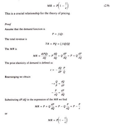
Marginal income is related to the price elasticity of demand by the following formula
Total revenue, marginal revenue and price elasticity:
We said that if the demand curve is falling, the TR curve will increase first, reach the maximum value, and then begin to decrease. You can use the previous derived relationships between MR, P, and e to establish the shape of the total revenue curve.
The total revenue curve reaches its maximum level at e=1.
MR = P (1 – 1/1) = 0
If E > 1, the total revenue curve has a positive slope, that is, it is still increasing, so if we consider the following, we have not reached its maximum point
P>0 and (1-1/E)>0; therefore Mr > 0
For E, 1, the total revenue curve has a negative slope, that is, it is falling.
P>0 and (1-1/E)<0;therefore Mr > 0
Then summarize these results as follows:
If the demand is inelastic (e<1), the increase in price leads to an increase in total revenue, and the decrease in price leads to a decrease in total revenue.
If the demand is elastic (e>1), the increase in price leads to a decrease in total revenue, and the decrease in price leads to an increase in total revenue.
If the demand has a single elasticity, then for e—1, then MR=0, so the total income is not affected by the change in price.
It is characterized in that. 24.1, we are giving individual seller or company supply curve. However, the market price is not determined by the supply of individual sellers.
Rather, it is determined by the total supply, that is, the supply that all sellers (or companies) offer collectively. This is an industry-wide supply. Thus, the industry supply curve shows the various amounts of products offered for sale by the industry at various prices at a particular time.
It is characterized in that. 24.1, we are giving individual seller or company supply curve. However, the market price is not determined by the supply of individual sellers. Rather, it is determined by the total supply, that is, the supply that all sellers (or companies) offer collectively. This is an industry-wide supply. Thus, the industry supply curve shows the various amounts of products offered for sale by the industry at various prices at a particular time.
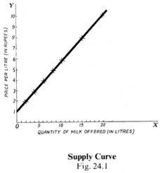
The amount that the industry can offer to sell depends on the price of its products in relation to the cost conditions of the enterprise. The cost conditions, in turn, depend on the price of the production or input factors used by the enterprise.
Short run supply curve:
"Short run" means the period when the size of the plant or machine is fixed, and the increase in demand for goods is satisfied only by the intensive use of a given plant, that is, by increasing the amount of fluctuating factors.
Under full competition, companies produce output where marginal costs are equal! Price - - - if the price is higher than the marginal cost, it will pay the company to expand its output so that it is equal to that price. On the other hand, if the price is less than the marginal cost, it is suffering losses and reduces its output until the marginal cost and price are equal. Therefore, the marginal cost curve of an enterprise is the supply curve of a company that is fully competitive in the short term.
But even in the short term, companies do not supply at a price below their minimum average variable cost. That is, in the short term, companies should at least try to cover their" variable costs." Thus, the short-term supply curve of the enterprise coincides with that portion of the short-term marginal cost curve that is above the minimum point of the short-term average variable cost (SAVC) curve.
The following figure [Fig. 24.2 (A)) makes it clear:
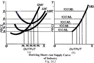
In this figure, it is a diagram. 24.2(a)is relevant to the enterprise, and 24.2 (b)is the supply curve for the industry. Let's first look at the diagram. 24.2(a) relates to a single company. Along the axis OX represents the output to be supplied, and along oy represents the price. SMC curve is the short-term marginal cost curve, and as mentioned above, it is the short-term supply curve of the company. However, only that part of the SMC curve above the short-range average variable cost (SAVC) means the thicker part above the dotted line.
So for price OP0, OM0 output is supplied, for OP1 price, OM1, quantity is supplied at OP2 price, OM2 is supplied, etc. The price below OP0 corresponds to the dotted part of the SMC below the minimum point of the SAVC (short-run average variable cost) curve, so nothing is supplied below the price OP.
Now, from the supply curve of the enterprise, let us derive the supply curve of the"whole"industry, in which every company is a constituent par) the supply curve of the industry SRS""is derived by the sum of the horizontal (i.e., addition to the horizontal) of that part of the marginal cost curve of all companies that are above the minimum point of their average fragile cost curve. It is believed that this industry consists of 100 identical companies, such as those shown in the figure. 24.2(a).
Long-term supply curve:
In the long run, it is considered to be a long enough period to allow for change in both the size of the factory and the number of companies in the industry. In the short term, the increase in demand is met by overuse of existing plants, while in the long term it is met not only by the expansion of existing plants, but also by the entry of new companies into the industry.
In addition, in the short term, companies have seen their marginal costs produce output equal to the price. But in the long run, the price must be equal to both marginal and average costs. The reason is that when all the companies in the industry are making normal profits, the industry will be in equilibrium and will only make normal profits if the price, i.e. average earnings (AR), is equal to the average cost AC.
The Shape of the supply curve depends, in the long run, on whether the industry follows the law of constant returns (i.e., constant costs) or is subject to a decrease in returns (i.e., an increase in costs) or an increase in returns (i.e., a decrease in costs). These curves are shown below.
Constant cost industry supply curve:
The supply curve for the constant cost industry is shown in the figure below (Fig. 24.3)

It is characterized in that. 24.3 (a) the LMC associated with the enterprise is a long-term marginal cost curve, and the LAC is a long-term average cost curve. They intersect at R, so at the point R, it means that the marginal cost is equal to the average cost. Here it is also equal to the price OP. So, in the output OM, MC=AC=Price.
Now look at the figure. 24.3(b). Corresponding to the OP price, the long-term supply curve is Lsc, which is a horizontal straight line parallel to The X-axis. This means that whatever the output along the X-axis, the price is the same OP where the marginal cost and the average cost are equal. Because it is a constant cost industry, the cost remains the same.
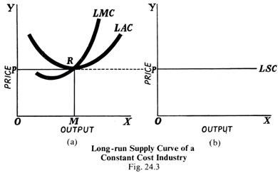
It is an industry in which the economy and uneconomic are offset so that the cost of production does not change, even if output increases (or decreases). Also, if new companies enter the industry to respond to increasing demand, they will not raise or lower the cost per unit.
Thus, the industry can supply any quantity of goods at a price OP equal to the minimum long-term average cost, which ensures normal profit to all companies engaged in the industry, that is, all companies will be in a long-term equilibrium: price=MC=AC. All companies have the same cost conditions.
Thus, for a continuing cost industry, the long-term supply curve LSC may be a horizontal line (i.e., perfectly elastic) within the price OP adequate to the minimum monetary value. This means that whatever the supplied output, the price will remain the same.
Increasing cost industry supply curve:
When the cost industry increases, the cost of production increases as existing companies expand or new companies enter the industry to respond to increasing demand. The external uneconomic outweigh the external economy. The increase in demand for production resources required to produce greater output to meet the increase in demand for products leads to higher costs of production and, as a result, its price increases.
The increase in cost shifts both the average cost curve and the marginal cost curve upwards, and the minimum average cost rises. This means that whether the additional supply comes from the expansion of existing companies or from new companies that may have entered the industry; the additional supply of products will be higher prices, all of which are shown in the following figure (Fig. 24.4).
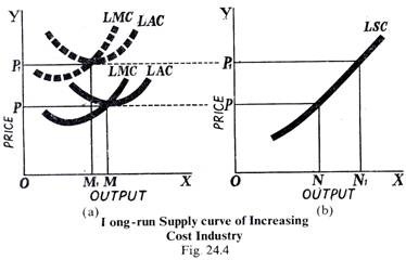
24.4(A) indicates the position of individual companies. The position of the dotted LMC and Lac curves indicates that they are shifting upward so that each company achieves a long-term equilibrium and the price OP,=MC=AC. But in the figure. In 24.4(B) on the industry, we can see that price OP i supplies more money ON1 than price OP (i.e., ON).
This means that the long-time supply curve LSC tilts upward to the right as the supplied output increases. That is, more will be supplied at a higher price. It can be seen that the long-term supply curve is tilted upward to the right when the cost industry increases, therefore, higher prices for scarce production resources to attract them from other uses so that production in this particular industry can be increased.
Cost-cutting industry supply curve:
In industries where costs decrease, costs decrease as production increases due to the expansion of existing companies or the entry of new ones. In this case, the economies of scale outweigh the uneconomic, if any. This happens when young industries grow in new regions, where the supply of productive resources is abundant. The net external economy pushes down the cost curve, allowing additional supply of output to come at a lower price.
The following figure (Fig. 24.5) clarifies the whole:
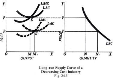
24.5(A) shows how the new, i.e. dotted LMC and Lac curves are shifting down from their original position when the lmc and LAC curves intersect at the E where all companies were in equilibrium and generating OM. Since the new curve intersects with E1, at this point, companies in the industry have achieved a long-term equilibrium, each producing OM, output, price OP=MC=AC. But look at the diagram. In 24.5 (B), we see that at the OP1 price, the ON is supplied more than or equal to the ON supplied by the original price OP.
LSC is right for cheaper supply of production resources, which means that additional supply of output is coming at a lower price since both marginal cost and average cost have fallen.
Summary:
Therefore, we can see that the short-term supply curve of the industry is always tilted upward to the right, but the long-term supply curve may be a horizontal straight line, inclined upward or downward, depending on whether the industry in question is a constant cost industry, cost industry increase or decrease cost industry. But the long-term upward slope curve is more typical of the real world.
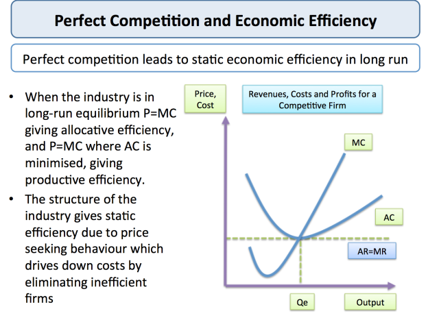
In free market, market cost reflect the complete s of resources and freedom of entry and exit, full access to information by all participants, homogeneous products and therefore the incontrovertible fact that nobody buyer or seller, or a gaggle of buyers or sellers, has any advantage over others.
Perfect competition is often used as a measure to match with other market structures, because it displays a high level of economic efficiency. Allocation efficiency:
We can see that within the short and future, the worth is adequate to the incremental cost (P=MC) and thus the allocation efficiency is achieved.
The ruling price maximizes the excess of consumers and producers.
No one can make better without making other agents a minimum of as worse–i.e. we achieve Pareto optimum allocation of resources.
Production efficiency:
Production efficiency occurs when balanced output is supplied at a minimum monetary value. This is achieved within the future for a competitive market.
Companies with higher unit costs might not be ready to justify remaining within the industry as market prices are pushed down by the force of competition.
Dynamic efficiency:
That is, there's little scope for innovation designed purely to differentiate products and permit suppliers to develop competitive advantages within the market and establish monopoly power.
Perfect competition-the chain of reasoning
Is perfect competition good for economic efficiency?
Some economists believe that perfect competition isn't an honest market structure for top levels of research and development spending and therefore the resulting product and process innovation.
Indeed, monopolistic or oligopolistic markets could also be simpler within the end of the day in creating an environment for research and innovation to flourish. Cost-cutting innovation from one producer is completed immediately, assuming perfect information, without transferring costs to all or any other suppliers.
That said, a competitive market would offer discipline for companies to regulate costs, minimize waste of scarce resources, set high prices and refrain from exploiting consumers by enjoying high profit margins. During this sense, competition can stimulate improvements in static and dynamic efficiency over time.
The future of perfect competition therefore exhibits an optimal level of economic efficiency. However, for this to be achieved, all of the conditions of full competition, including the relevant market must hold.
A. Short run
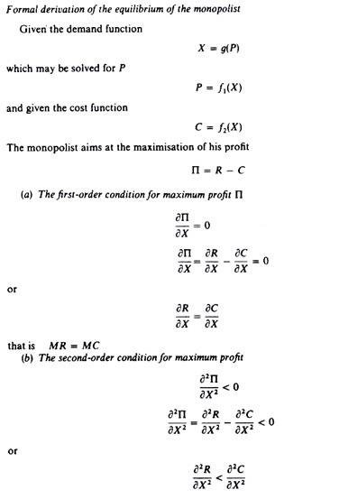
A monopolist maximizes his short-term profits if the following two conditions are met first, MC equals Mr. Secondly; the slope of MC is larger than that of Mr at the intersection.
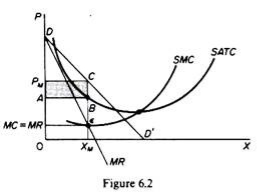
In Figure 6.2, the equilibrium of the monopoly is defined by the point θ at which MC intersects the MR curve from below. Thus, both conditions of equilibrium are met. The price is PM and the quantity is XM. Monopolies realize excess profits equal to shaded areas APM CB. Please note that the price is higher than Mr
In pure competition, the company is the one who receives the price, so it’s only decision is the output decision. The monopolist is faced with two decisions: to set his price and his output. But given the downward trend demand curve, the two decisions are interdependent.
Monopolies set their own prices and sell the amount the market takes on it, or produce an output defined by the intersection of MC and MR and are sold at the corresponding price. An important condition for maximizing the profits of monopolies is the equality of the MC and the MR, provided that the MC cuts the MR from below.

We can now revisit the statement that there is no unique supply curve for the monopolist derived from his MC. Given his MC, the same amount could be offered at different prices depending on the price elasticity of demand. This is graphically shown in Figure 6.3. Quantity X is sold at price P1 if demand is D1, and the same quantity X is sold at price P2 if demand is D2.
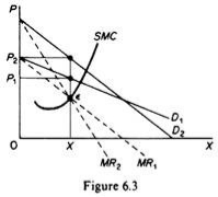
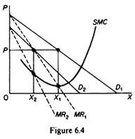
So there is no inherent relationship between price and quantity. Similarly, given the monopolist MC, we can supply various quantities at any one price, depending on the market demand and the corresponding MR curve. Figure 6.4 illustrates this situation. The cost condition is represented by the MC curve. Given the cost of a monopolist, he would supply 0X1 if the market demand is D1, then p at the same price, and only 0X2 if the market demand is D2 B.Long-term equilibrium:
In the long run the monopolist will have time to expand his plants or use his existing plants at every level to maximize his profits. However, if the entry is blocked, the monopolist does not need to reach the optimal scale (that is, the need to build the plant until the minimum point of LAC is reached), neither does the guarantee that he will use his existing plant at the optimum capacity. What is certain is that if he makes a loss in the long run, the monopolist will not stay in business.
He will probably continue to earn paranormal benefits even in the long run, given that entry is banned. But the size of his plant and the degree of utilization of any plant size depends entirely on the market demand. He may reach the optimal scale (the minimum point of Lac), stay on the less optimal scale (the falling part of his LAC), or exceed the optimal scale (expand beyond the minimum LAC), depending on market conditions.
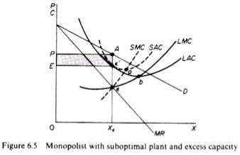
Figure 6.5 shows when the market size does not allow the monopolist to expand to the minimum point of Lac. In this case, not only is his plant not optimal (in the sense that the economy of full size is not depleted), but also the existing plant is not fully utilized. This is because on the left of the minimum point of the LAC, the SRAC touches the LAC at its falling part, and the short-term MC must be equal to the LRMC. This happens in e, but the minimum LAC is b,and the optimal use of the existing plant is a. Since it is utilized at Level E', there is excess capacity. Finally, figure 6.7 shows a case where the market size is large enough for a monopolist to build an optimal plant and be able to use it at full capacity.
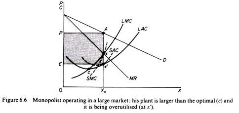
In Figure 6.6, the scale of the market is so large that monopolists have to build plants larger than the optimal ones to maximize output and over-exploit them. This is because to the right of the minimum point of LAC, SRAC and LAC is tangent at the point of positive slope, and SRMC must be equal to LAC. Thus, plants that maximize the profits of monopolies are, firstly, larger than the optimal size, and secondly, they are over-utilized, which leads to higher costs. This is often the case with utility companies operating at the state level.
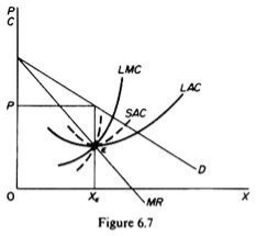
It should be clear that which of the above situations will appear in a particular case will depend on the size of the market (given the technology of monopolists). There is no certainty that monopolies will reach their optimal size in the long run, as is the case with purely competitive markets. In Monopoly, there is no market force similar to those of pure competition that will lead companies to operate at optimal plant size in the long run (and utilize it at its full capacity).
The supply curve under incomplete competition or Monopoly is not unique.
This is due to the fact that, unlike full competition, the price is determined simultaneously with the volume of goods produced, and the price is not given to the enterprise under monopoly or Monopoly competition.
Here the company is the price manufacturer of her products. Therefore, the company fixes the price at which it will get the maximum profit. The supply of goods is determined by the market demand for its products. Therefore, it is impossible to talk about the supply curve under monopoly or Monopoly competition.
The output supplied by the producer under such exclusive circumstances depends on the market demand conditions of his product and draws a unique supply curve (and supply schedule).
Therefore, it is not quite applicable to the causes of incomplete competition, monopoly competition, monopolies and oligopolies. This is because the concept of the supply curve refers to questions about the amount of goods a company supplies at various given prices.
Under various sorts of incomplete competition, individual companies don't take the worth as given and aren't mere quantity adjusters. In fact, under various forms of incomplete competition, the company sets its own prices. For companies under incomplete competition, it is not a matter of adjusting output or supply at a given price, but choosing a combination of price output that maximizes profit.
Commenting on the relevance of the supply curve, professor Baumol writes: the supply curve is, strictly speaking, a concept usually relevant only in the case of pure (or complete) competition...The reason for this lies in its definition—the supply curve is designed to answer the form question, “to answer the form question how much would solidify the supply if it encounters a price that is fixed in P dollars. But such questions are most relevant to the behavior of companies that actually deal with prices.”
Monopoly
Monopolies exist when a particular enterprise is the sole supplier of a particular commodity. Monopoly has little to no competition when producing good or service. Monopolies are entities that have significant market power (the power to charge high prices).
Inefficiency in Monopoly
In monopolies, the company sets a certain price for the goods that are available to all consumers. The quantity of good things will be less, and the price will be higher (this is what makes good things a commodity). Monopoly pricing creates a burden loss because companies forgoes transactions with consumers. The burden loss is a potential gain that hasn't gone to producers or consumers. As a result of the loss of burden, the combined surplus (wealth) of monopolies and consumers is less than that obtained by consumers in competitive markets. Monopolies are less effective in total profits from trade than in competitive markets.
Monopolies can become inefficient and less innovative over time, because they do not have to compete with other producers in the market. For private monopolies, complacency can overcome barriers to entry and create room for potential competitors to enter the market. In addition, long-term alternatives in other markets can take control when monopolies become inefficient.
Market failure
If the market is unable to allocate resources efficiently, a market failure occurs. In the case of monopolies, abuse of power can cause market failure. Market failure occurs when the price mechanism does not take into account all of the costs and/or benefits of providing and consuming goods. As a result, the market is not able to supply socially optimal quantities of goods. Monopolies are imperfect markets that limit output in an attempt to maximize profit. Monopoly market failure can happen because enough of the great isn't made available and/or the worth of the great is just too high. Without the presence of competitors in the market it can be a challenge for monopolies to self-regulate and remain competitive over time.


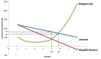
In economics, weight loss is a loss of economic efficiency that occurs when the equilibrium of goods or services is not Pareto optimal. If good or service is not the optimal Pareto, economic efficiency is not equilibrium. As a result, when resources are allocated, it is impossible to make any individual better, without worsening at least one person. When weight loss occurs, there is a loss in the economic surplus in the market. Weight loss means that the market cannot be cleared naturally.
Causes of loss of dead weight
The loss of a dead weight is the result of a market that cannot be cleared naturally and is therefore an indicator of market inefficiency. Supply and demand for goods or services are not balanced. The causes of weight loss are:
- Imperfect market
- Externality
- Taxes or subsides
- Price ceiling
- Price floor
Dead Loss decision
To determine weight loss on the market, the formula P=MC is used. The loss of the dead weight is equal to the change in price multiplied by the change in the required quantity. This formula is used to identify the causes of inefficiencies in the market.
For example, in a nail market where the cost of each nail is$0.10, demand decreases from high demand for cheap nails to zero demand for nails at$1.10. In a fully competitive market, producers will charge$0.10 per nail, and every consumer whose marginal profit exceeds$0.10 will have a nail. But if one producer has a monopoly on nails, they charge a price that brings the maximum profit. If they charge$0.60 per nail, all parties that have less than$0.60 of marginal gains will be excluded. If equilibrium is not achieved, the parties that would have entered the market with pleasure are excluded for non-market prices.
.Sometimes policymakers impose binding constraints on items if they believe that the benefits from the transfer of surpluses outweigh the negative effects of the loss of burdens.
In pure price discrimination, the seller charges the customer a different price for the same product or service based on what the seller believes can get the customer to agree on, the vendor charges each customer the utmost price he or she is going to pay.
Types of discrimination monopolies:
Price discrimination is the following three types:
1. Personal price discrimination:
For example, doctors charge different fees for the same surgery from rich and poor patients.
2. Geographical price discrimination:
Under Geographical price discrimination, monopolies charge different prices in different markets for the same product. It also includes dumping, which allows producers to sell the same goods at home at one price, and abroad at another.
3. Price discrimination according to usage:
When monopolies charge different prices for different uses of the same product, it is called price discrimination according to use.
Conditions for price discrimination:
For price discrimination to exist, basic conditions are required.
These are:
1. Difference in the elasticity of demand:
Price discrimination is feasible only the elasticity of demand is different in several markets. Monopolies will fix higher prices where demand is inelastic and lower prices where demand becomes elastic. In this way, he will be able to increase his total income.
2. Market flaws:
In general, price discrimination is possible only if there is a certain degree of market deficiencies. Individual sellers can divide the market into separate parts only if it is incomplete.
3. Differentiated products:
Price discrimination is possible if buyers need the same services in relation to differentiated products. For example, Railways charge different rates for the transport of coal and copper.
4. Legal system:
In some cases, price discrimination is legally sanctioned. As the power board charges low power for domestic use, the best quotient.
5. The presence of monopoly:
Price discrimination is also called discrimination monopoly. It is clear that price discrimination is possible only under the conditions of monopoly.
Degree of price discrimination:
A.C.Professor Pigou has given the following three degrees of discrimination:
1. First-class price discrimination:
First-degree price discrimination is said to exist when a monopolist can sell each separate unit of his product at different prices. It is also known as full price discrimination. In the case of first-degree price discrimination, the seller charges a price equal to what the consumer is willing to pay. It means that the seller does not leave the consumer surplus to the consumer. Away from the top, under complete price discrimination, as under a simple monopoly, the buyer's demand curve will be the seller's marginal revenue curve.
2. Second-class price discrimination:
In the second-degree buyer price discrimination is divided into different groups, and from different groups will be charged different prices, which is the lowest demand price of that group. This type of price discrimination occurs when an individual buyer has had a demand curve that is completely elastic for the Good below and above a particular price.
3. Third time price determination:
Three-degree price discrimination is said to exist when a seller splits his buyer into two or more sub-markets and charges different prices from each group. The price charged in each sub-market depends on the output sold therein sub-market, alongside the demand conditions of that sub-market. In the real world, it's three times price discrimination that exists.
Given below can explain the major differences between the three markets
Perfect competition is a concept in microeconomics that describes a market structure that is completely controlled by market forces. If these forces are not met, the market is said to have incomplete competition.
There is no market that clearly defines full competition, but all real world markets are classed as incomplete. That is, perfect markets are used as a standard that can measure the effectiveness and efficiency of real world markets.
Perfect competition:
1. An outsized number of buyers and sellers.
2. Perfect competition among sellers.
3. Homogeneous products.
4. Lack of control over the factors of production.
5. Lack of price controls
6. Complete knowledge of the market.
7. One price or an equivalent price prevails everywhere.
Imperfect competition
Incomplete competition occurs in a market when one of the conditions of a fully competitive market is left unfulfilled. This type of market is very common. In fact, every industry has some type of incomplete competition. This includes various products and services, prices that are not set by supply and demand, competition for market share, buyers who do not have complete information about products and prices, and high barriers to entry and exit.
Incomplete competition is found in the following types of market structures: monopolies, oligopolies, monopolies, and oligopoly.
In monopolies, there is only one (dominant) seller. The company offers products to markets where there are no substitutes. Monopolies have high barriers to entry and there is a single seller who is a price maker. That means the company sets the price at which the product is sold regardless of supply or demand. Finally, the company can change the price at any time without notifying the consumer.
In oligopolies, there are many buyers, but only a few sellers. Oil companies, grocery stores, mobile phone companies, and tire manufacturers are examples of oligopolies. As there are few players dominating the market it may block others from entering the industry. Companies with this market structure can do so if they set prices for products and services in bulk or, in the case of cartels, take the lead.
Imperfect competition:
1. Little number of buyers and sellers.
2. Incomplete competition of sellers.
4. Artificial restrictions on production factors.
5. The presence of control.
6. Ignorance of purchase.
7. Price discrimination.
Monopoly:
1. Just one seller.
2. Lack of competition.
3. There's no product differentiation.
4. Artificial restrictions on production factors.
5. Full control of price.
6. Incomplete knowledge of the market.
7. Price discrimination.
Years ago in 1920s, the classical theory of price included two main models: pure competition and monopoly.
The double occupancy model was considered an intellectual exercise, not a real world situation. The general model of economic behavior from Marshall to Knight was pure competition.
In the late 1920s, economists became increasingly frustrated with the use of pure competition as an analytical model of business behavior. It was clear that pure competition could not explain some empirical facts.
Moreover, the practice of advertising and other sales activities can not explain the widely used businessman pure competition. Finally, as we predict when a pure competitive model will continuously reduce costs, companies have expanded their output with reduced costs, but never grow infinitely large.
In particular, it was this last fact of falling costs that created discontent and caused a widespread reaction to pure competition theory. This discontent caused a long series of debates and the publication of numerous articles that formed the “great cost controversy of the 1920s.
The earliest summary of the cost controversy should be found in Piero Sraffa's article. Sraffa pointed out that the falling cost dilemma of classical theory can be theoretically solved in various ways by introducing a demand drop curve for individual companies, a general equilibrium approach that appropriately incorporates the shift in costs induced by external economies (firms and industries), or by introducing a U-shaped sales cost curve into the model.
Of these solutions, Sraffa was the first to adopt, that is, a model with a negative personal demand curve that was more operationally and theoretically more plausible. The same line is a work published in 1933, in which E.It was adopted independently by Chamberlin and Joan Robinson.
It should be noted that both writers arrive at the same solution for enterprise and market equilibrium, but their analytical approach and methodology are quite different.
Assumption:
The fundamental assumption of Chamberlin's horde model is the same as that of pure competition except for the homogeneous product.
It can be summarized as follows:
- The seller's products are differentiated, but they are close replacements to each other.
- Entry and exit of companies in the group is free.
- . The company's goal is to maximize profits both in the short and long term.
- Factors and the price of technology are given.
- The company is assumed to behave as if it knows the demand and cost curves for sure.
- A long run consists of several identical short periods, which are assumed to be independent of each other, in the sense that the decision of a certain period does not affect the future period and is not affected by past actions. An optimal decision for one period is an optimal decision for another. Thus, by assumption, the maximization of short-term profits implies the maximization of long-term profits.
This requires that consumer preferences be evenly distributed among sellers with different tastes, and that differences between products do not create a difference in cost. Chamberlin himself realizes that the"heroic"assumptions are unrealistic, and he relaxes them at a later stage.
Short-term equilibrium:
The number of companies in the industry is fixed because existing companies cannot leave or new ones can enter.
Its conditions:
The company is in equilibrium when it is earning the maximum profit as the difference between its total revenue and total cost. For this purpose, it is essential that the two conditions must be satisfied: (1)MC=MR and (2)MC curves must cut the MR curve from the bottom at the equivalence point, and then rise upwards.
The price at which each company sells its output is set by the market forces of supply and demand. Each company will be able to sell as much as selected at its price. However, due to competition, it can not be sold at all at a price higher than the market price. So the demand curve for the company will be horizontal at that price, so the company’s P=AR=MR.
1. Marginal revenue and marginal cost approach:
The short-term equilibrium of the enterprise can be explained not only with the help of marginal analysis, but also with the help of total cost-total revenue analysis. At first, the limit analysis was carried out under the same cost condition.
This analysis is based on the following assumptions:
1. All companies in the industry use homogeneous production factors.
2. Their cost is equal. Therefore, all cost curves are uniform.
3. All companies have equal efficiency.
4. All companies sell their products at the same price, determined by the supply and demand of the industry, so that the price of each company is equal to AR=MR.
Determining equilibrium:
Given these assumptions, we assume that the price OP in the competitive market for the products of all companies in the industry is determined by the equivalence of the demand curve D and supply curve S at Point E in Figure 1(A), and that the average revenue curve(AR)coincides with the marginal revenue curve(MR).
When equilibrium is at point L in the panel (B) of the figure where (i) SMC is equal to MR and AR and (ii) SMC curve cuts the MR curve from below. Each company will produce OQ output and earn a normal profit at the maximum average total cost QL. When the MR curve is tangent to the SAC curve at its minimum point, the company is getting a normal profit. If the price is higher than these minimum average total costs, each company will earn a super-regular profit. Suppose that the price rises to OP2, and the SMC curve devalues the new marginal revenue curve MR2 (=AR2) from below at point A, and is now at the equilibrium point. In this situation, each company produces OQ2 output and earns a super-regular profit equal to the area of the rectangular P2ABC.
If the price falls below OP1, the company will make a loss because the SAC will be higher than the price. In the short term, we will continue to produce and sell OQ1 output at OP1 prices as long as we cover AVC. So, S is the shutdown point at which the company has a maximum loss equal to SK per output unit. If the price falls below OP1, the company will be closed because even the minimum average variable cost cannot be covered. So OP1 is the shutdown price.
From the above discussion, we may conclude that in the short term, each company may be making either ultra-regular profits, or normal profits or losses, depending on the price of the product.
2. Total cost revenue analysis:
The short-term equilibrium of the enterprise can also be shown with the help of the total cost and the total revenue curve. The company can maximize profit at the output level, where the difference between total revenue and total cost is the greatest. This is shown in Figure 2.TR is the total revenue curve; TC is the total cost curve.
This is because the company sells small or large quantities of products at a constant price under perfect competition. If the company does not produce anything, then the total income will be zero. The more it is produced, the greater the increase in total revenue. Thus, the TR curve is linear and inclined upwards.
The company maximizes profits at output levels where the gap between the TR and TC curves is greatest.
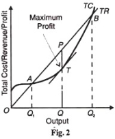
In Figure 2, the maximum amount of profit is measured by TP at the OQ output. With a smaller or larger output than oq between A point and B point, the company's profit shrinks. If a company produces an OQ1 output, its loss is maximum because the TC curve is above the TR curve. In Q1, that profit is zero. A similar situation prevails in Q2
Since marginal revenue is equal to the slope of the total revenue curve and marginal cost is equal to the slope of the tangent of the total cost curve, if the slope of the total cost curve and the revenue curve is equal to p and T, then the marginal cost is equal to the marginal revenue. It is clear that the point of maximum profit lies in the area of maximum losses: the rise in marginal costs (if TC is below TR) and the fall in marginal costs (if TC is above TR).
Explaining a company's equilibrium using the total cost-revenue curve doesn't throw more light than is provided by marginal cost-marginal revenue analysis. This is useful only in the case of a specific limit determination where the total cost curve is linear over a particular output range.
But that makes the balance of the enterprise a laborious and difficult analysis, especially when we have to compare changes in costs and revenues resulting from changes in production volumes. In addition, you can not know the maximum benefit at once. For this, you need to draw several tangents, which is a real difficulty.
Corporate long-term equilibrium:
In the long term, it is possible to make more adjustments than in the short term. The company can adjust the capacity and scale of the operation plant to the modified circumstances. Therefore, all costs are variable. Companies need to get only the usual profit. If the price is above the long-term AC curve, companies will get paranormal benefits.
Attracted by them, new companies enter the industry and compete for Paranormal profits. If the price falls below the LAC curve, companies will incur losses. As a result, some companies will leave the industry so that companies do not earn more than their usual profits.
Thus, "long-term companies are in equilibrium when they have adjusted their factories to produce at the minimum point of the long-term AC curve (at this point) bordering the demand (AR) curve defined by the market price".
Assumption:
This analysis is based on the following assumptions:
1. Companies are free to enter or leave the industry.
2. All companies have equal efficiency.
3. All factors are homogeneous. They can be obtained at a certain uniform price.
4. The cost curve of the enterprise is uniform.
5. Corporate factories are equal in giving technology.
6. All companies know about the price and output to output.
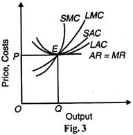
We assume equal costs for all companies in the industry, so all companies will be in equilibrium in the long run. At OP prices, companies will have no tendency to leave or enter the industry, and all companies will have a normal profit.
Professor Chamberlin's description of the theory of excess capacity differs from the theory of ideal output under perfect competition.
Its output is ideal and there is no extra capacity in the long run. Under monopolistic competition, the company's demand curve is tilted downward due to product differentiation, so the company's long-term equilibrium is to the left of the minimum point on the LAC curve.
The Tangent point between the demand curve and the LAC curve of the enterprise will lead to “ideal output" and excess capacity.
Assumption:
The Chamberlin concept of excess capacity assumes the following:
(i) A large number of companies;
(II) Each produces a similar product independently of others;;
(III) It can meet the low price and attract other customers, and will lose some of the customers by raising the price;
(IV) The preferences of the "consumer" are fairly evenly distributed among products of different varieties;
(V) No company has an institutional monopoly on the product;
He gives the following reasons for such situations:
(I) the enterprise may consider costs more than demand when fixing prices.
(II) Can aim at ordinary profit instead of maximum profit,
(iii) They can follow the policy of “let live and live" and cannot resort to price cuts.
(iv) They may have formal or implicit contracts, open price associations, trade association activities and price maintenance in the construction of esprit de corps.
(v) The dealer by the manufacturer may have an even price imposition.
(vi) Companies may resort to excessive differentiation of their products in an attempt to deflect attention from price reductions.
(vii) Business or professional ethics prevents companies from resorting to aggressive price competition.
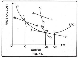
Equilibrium in the absence of price competition
In the absence of price competition due to the prevalence of these factors, the curve dd is insignificant, and companies are only interested in the group DD curve. Suppose that there is an initial short-term equilibrium in S where the company is earning supernormal profits because the price OP corresponding to Point S is above the LAC curve.
With the entry of new companies in the group, ultra-normal profits will compete. The new company splits the market, and the DD curve is pushed to the left, as in D1d1 in Figure 18, it touches the LAC curve at point A1, but this point A1 is a stable equilibrium without price competition for all the companies in the group, earning only normal profits. Each company produces and sells OQ output at QA (=OP) price.
In Chamberlin's analysis, O1 is the "ideal output". However, each company in the group produces OQ output in the absence of price competition. Thus, OQ1 represents excess capacity under non-price Monopoly competition.
Chamberlain concludes that if prices do not fall for a long time under non-price competition and costs rise, the two are equated by the development of excess capacity without automatic correction. Such excess capacity can develop under pure competition due to miscalculations on the part of producers and sharp changes in demand and cost conditions.
But under monopolistic competition, prices always cover costs and can become permanent and normal by price competition not working. Surplus capacity is never abandoned, and the result is a high price and waste. They are a waste of monopolistic competition.
Significance of excess capacity:
The concept of excess capacity has a very practical significance. Professor Caldor characterizes it as “intellectually impressive”, “very original"and"revolutionary doctrine".’
1. This shows the unconventional possibility that increased supply can lead to higher prices. The “waste of competition “that has been a mystery has been unfolding. They relate to monopolistic competition, not full competition, as strongly implied by previous economists.
2. It establishes the truth of the proposition that perfect competition and an increase in returns are incompatible, and proves that falling costs will eventually lead to monopoly or Monopoly competition when Monopoly competition prevails, the number of companies will grow. But each company will be smaller in size than under full competition.
3. This involves the wasteful use of resources by fostering less efficient enterprises. Such companies may employ more human resources, equipment and raw materials than necessary. This leads to excess or unused capacity.
Here are certain reasons that have led to the emergence of oligopolies. These are:
1. Large-scale investment of capital:
The number of companies in the industry may be small due to the large requirements of capital. Entrepreneurs will not want to bet heavily on an industry that, in addition to output to existing ones, is likely to push prices down.
In addition, newcomers may be afraid to provoke a price war by existing companies in the industry. It is always true that in the midst of differentiated products, it is difficult to make a new product.
2. Managing essential resources:
Few companies control some indispensable resources that may allow them to secure several benefits in cost over all others or this allows them to operate advantageously at a price that others cannot survive.
3. Legal restrictions and patents:
In the Public Works sector, the entry of new enterprises is closely regulated by the granting of certificates by the state. This policy of elimination of rivals may be due to small-scale uneconomic or duplication of services. Another factor for the emergence of oligopolies is the patent rights that some companies acquire in matters of some goods.
4. Economies of scale:
Another factor that causes the emergence of oligopolies is large enterprises. In some industries, some companies can meet the entire demand for products. Many companies are likely to meet demand, and small businesses may not be able to secure an economy of large production. In those industries where there is a lot of mechanization and there is quite a large economy, a small number of companies will survive.
Companies achieve such a huge size that some of them can meet the overall demand. For example, automobile, steel industry, petroleum etc. Oligopolies can also be found in local markets. In small towns, some companies may be enough to meet the demand, for example, gasoline, banks, suppliers of building materials. The market is small, and therefore some companies can be satisfied.
5. Outstanding entrepreneurs:
In some industries, some excellent entrepreneurs whose cost is lower than inferior rivals sell under these entrepreneurs, eliminating most of the rivals.
6. Merger:
The main motives of the merger include increased market power, more resources, economies of scale, and market expansion.
7. Difficulties in entering the industry:
Finally, oligopolies can exist due to the difficulty of entering the industry. One big difficulty in some industries is the large requirements for capital. Businessmen do not like to venture into those industries, even of one company, could push down prices to such an extent that makes it unprofitable for all. They may also be afraid of the price war their entry might cause from existing companies in the industry. Also, in the presence of an already established and well-established brand, the difficulty of marketing a new product or a new brand can lead to future participation in the industry.
Cooperative and prisoner dilemmas
Coordinated action in oligopolies is a situation in which the enterprise decides jointly maximizes the price and output and their joint profit. This situation is called
Collusion in this situation, if there is a defect; it will be beneficial to one enterprise.
Unless others do, they will undercut prices and raise output. Uncooperative behavior is a situation in which they do not decide to cooperate their price and output separately, compete with each other. That company Oligopolies do not cooperate it is called uncooperative equilibrium or NASH Equilibrium (named after the American mathematician John Nash).
In oligopolies, the basic dilemma facing companies is whether to cooperate or not
Compete. If they cooperate, the profit will be maximum; otherwise the profit will be maximum decrease for all. Now we will see the actions of oligopolistic companies
Through the example of Game Theory. Game theory is the study of decision making
Making in strategic interaction (movement and countermoves) situations)
It occurs among rival companies. We assume the case of only two companies
Market called double occupancy
This is called the payoff matrix of two company’s double-occupancy game.
The numbers on the right of each cell show the company A and the profit on the left
The numbers in each cell indicate the profit of the Company B(in Rs. Project report). It can explain that if the two companies cooperate and produce half of the market share each will earn Rs. 20crores of profit. In case of cooperation they can
Maximize their profits. If Firm A defects and produces two-thirds of the output、
Company B produces half of the exclusive output, and Company A gets Rs. 22 cloughless and Company B Rs. 15 if the company produces a defect of B and a second-third as well as clowless.
And company A produces half, and Company B wins Rs. 22 crawl and company A
You only earn Rs. 15 if crowless both compete and decide to produce two-thirds
Market Structure.
Each of the exclusive output, the profit for both falls on Rs. 17 crawless this
What kind of game they reach uncooperative solutions when they can c .Two prisoners Mr Lamb and Mr Sham have been arrested for committing a crime
And interrogated separately. They are said to be:
A) If both are claimed to be innocent, they will get a lighter sentence which is 1
Years in prison.
B) If one confesses and the other does not, who will confess freely released, others are punished for 9 years of imprisonment, and
C) If both confess both will receive a punishment of 6 years in prison.
The payoff matrix shown in Table 12.2 shows the prisoner's dilemma about whether to confess or not to confess. If none of them confess, both get 1 year of prison, but Ram confesses, and if Shyam does, Ram will left free, Shyam will get a 9-year prison sentence and Vise-vice versa. And then if both confess, both get 6 years in prison. No Confession is the best solution in this game (Pareto efficient solution), but this
Always leave in uncertainty. This solution is not a stable solution as one
If he/she does not confess, he / she get 9 years imprisonment, and the other does not.
Thus, confession reigns in the minds of both prisoners. Both cases
They then confess they both end up in prison for 6 years. This kind of
Equilibrium is called Nash equilibrium. It is clear from both numbers above
It is that they cooperate; they can get the maximum benefit than if
Compete.
Types of cooperative behavior
To avoid uncertainty arising from interdependence and to avoid price
Cutting wars and throat competition, companies under oligopolies often get into some agreement on determining the uniform price and output. The contract is as follows of the following two types.
Explicit collusion: This is a situation where an oligopolistic company officially does
(Explicit) matching to determine and maximize uniform pricing and output
Their joint interests. Such an agreement at the international level is called a cartel,
Many such contracts have been made in the past. Best example of
The cartel is that of the OPEC-organization of oil exporting countries.
Since 1973, Saudi Arabia and others have formed the cartel. Anne.
Individual companies always have the incentive to cheat. There is a possibility of cheating if the number of companies is large, it will be large. There is very few misconduct by small companies.
Impact on market prices.
Implicit cooperation: when companies cooperate without explicit cooperation
Agreement it is called tacit cooperation.
Oligopolies: prices and Output decision
Company a produces half of the exclusive output that company B expects to do
Same and Company B do not do so because they achieve cooperatives
Types of uncooperative behavior
In the absence of a formal or informal agreement on cooperation, the enterprise
Compete with each other under oligopolies. Uncooperative or competitive
Actions under oligopolies can be of the following types:
- Competition for market share: companies under oligopoly always compete with Each other for market share. They use various forms of non-price competition. Such as advertising, quality products etc. To increase their market share. For Examples of major mobile service providers in Delhi such as Airtel, Hutch and Idea competed to increase their mobile connection.
2. Secret cheating: in oligopolies, because of huge market share, companies sell their products by contract. Large-scale production and distribution is done through the contract. When companies offer them secret discounts or rebates if a hidden fraudulent act is discovered called an increase in sales to the buyer.
3. Competitive markets and potential entrants: The theory of competitive markets explains that in the long term, the extraordinary profits earned by oligarchs can be eliminated without actual entry. Potential entry could also affect the market as much as the actual entry. This is possible only in the following two cases conditions are met:
- Entry should be easy to achieve: there should not be any barriers entries were created by nature or company.
- Price while having to think about existing companies
4. And output decisions: existing companies must react when new companies try entering the market. We have to cut them down to limit new comers (short-term). Competitive markets always expect potential entry for huge profits
It was acquired by existing companies in the market. But the entry into such markets also the cost of fixed costs is very high. To develop, design and sell new products such a market involves huge sunk costs. Sunk costs are those costs you can't it will be recovered if the company leaves the market immediately. Companies that produce more than one company and among these costs to discriminate of products many Product. For new companies produce a huge number of differentiated products it's not simple, therefore, these costs are very high for companies that produce a single products in the market. If a new company can enter and leave the market without any sunken cost of entry, such a market is called a fully competitive market. The market is as follows’
In these cases, companies are fully contestable, even if they have to pay some cost of entry.
Costs are recouped when companies leave the market. If the Sunk Cost is lower, the market will be more contestable and Vise-vice versa. The sunken cost of entry that constitutes an entry barrier. The higher the sunk cost, the greater the will be the profit earned by the existing enterprise. If the enterprise operates in the market did not enter the larger sinking costs had a big revenue. As part. The strategy covers existing companies’ always lower prices as much as possible Total cost. New companies if they charge higher prices and get extraordinary profits you may enter and capture profits. Compel existing companies to compete to keep prices low. The threat of entry into the market is as effective as it really is Entry to limit profiteering by existing companies.
References
Https://opentextbc.ca/principlesofeconomics/chapter/8-1-perfect-competition-and-why-it-matters/
Https://www.economicsdiscussion.net/articles/short-run-and-long-run-supply-curves-explained-with-diagram/1677
Https://pressbooks.bccampus.ca/uvicecon103/chapter/4-4-elasticity-and-revenue/
Https://www.tutor2u.net/economics/reference/perfect-competition-assumptions-and-characteristics
Https://courses.lumenlearning.com/suny-microeconomics/chapter/efficiency-in-perfectly-competitive-markets-2/
Https://www.economicsdiscussion.net/monopoly/constructing-a-supply-curve-under-monopoly/17069
Principles of Microeconomics
Timothy Taylor, Saint Paul, Minnesota
Steven A. Green law, Fredericksburg, Virginia
Microeconomic theory Andreu Mas-Colell
Principles of Economics N. Gregory Mankiw