UNIT 3
Price output decisions under different market conditions
Perfect and imperfect competition price and output decision
Equilibrium refers to when the firm has no inclination to expand or to contract its output. The producer can attain equilibrium under two situations.
2. Imperfect competition – Under this condition, the firm has the freedom to set prices for their output. Price is not constant here, as the firm adopt independent pricing policy.
The Marginal Revenue-Marginal Cost Approach
Profit depends on revenue and cost. Thus equilibrium revolves around revenue and cost. According to the MR-MC approach, a producer is said to be in equilibrium when:
- A Firm can maximise the profit when marginal revenue is equal to marginal cost.
- MR is the addition to TR from the sale of one more unit.
- MC is the addition to TC when an additional unit is produced.
- Thus when MR = MC, TR-TC result in maximum profit.
- If MR exceeds MC, then producer will produce more as it adds to the profit.
2. MC is greater than MR after the MC=MR Output Level
Producer’s Equilibrium when Price remains Constant
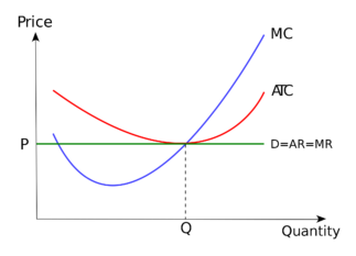
Price remains constant under conditions of perfect competition. Here price is equal to AR. When price is constant, revenue from each additional unit is equal to AR. It means AR curve is same as MR curve. The firm attains equilibrium when two condition are fulfilled , that is firm aims at producing that level of output at which MC is equal to MR and MC is greater than MR after MC = MR output level.
Producer’s Equilibrium when Price is not constant
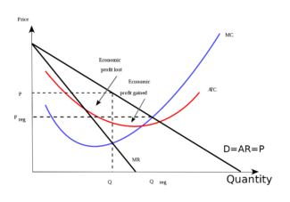
When there is no fixed price, price falls with an increase in output. The producer sells more units at a lower price. In this case MR slopes downwards. The firm aims at producing that level of output at which MC is equal to MR and MC is greater than MR.
Short run and long run supply curves
Supply curve shows the relationship between price and quantity supplied. According to Dorfman, “Supply curve is that curve which indicates various quantities supplied by the firm at different prices”.
Supply curve can be divided into two parts as:
Short run supply curve of a firm
Under Short run , fixed cost remains constant, supply can be changed by changing the only the variable factors. Thus the firm has to bear fixed cost id it is shut down. Thus in short run, goods are supplied at price is either greater or equal to average variable cost. Average revenue is equal to marginal revenue under perfect competition. Hence the firm will produce at the point where marginal revenue and marginal cost are equal.
Prof. Bilas has defined it in simple words, “The Firm’s short period supply curve is that portion of its marginal cost curve that lies-above the minimum point of the average variable cost curve.”
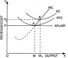
From the above figure we can see that, the firm will not be covering its average variable cost, at price less than OP. At price OP, OM is the supply. MC and MR cut at point A, OM is equilibrium output. If price rise to OP1, the firm will produce OM1 output. This short run supply curve of a firm starts from A upwards i.e., thick line AB.
Long run supply curve
Under long run, the supply curve changes by changing all the factors of production. The firm produces only at minimum average cost in long run. In this case, long run marginal cost, marginal revenue, average revenue and long run average cost are equal. The firm enjoys normal profit.
Optimum production is the point where minimum average cost is equal to marginal cost. Long run supply curve is a portion where marginal cost curve that lies above the minimum point of the average cost curve.
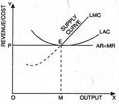
Optimum point is the Point E, as at this point MR=LMCAR minimum LAC. The portion of LMC above point E is called long run supply curve
Price determination under Perfect competition:
The equilibrium price refers to that price at which the demand and supply of a commodity are in equilibrium (equal). In other words Quantity demanded is equal to Quantity supplied. Once equilibrium price is reached here is no tendency for the price to move upward or downwards.
According to Marshall both Demand and Supply are essential in determination equilibrium price. Like the two blades of a scissor that cut piece of paper, demand and supply are important part in determining equilibrium price. Both the blades are useless when they are applied individually. Thus demand and supply are equally important in determining equilibrium price.
This can be explained with the help of following table:
Price (Rs.) | Quantity Demanded (Units) | Quantity Supplied (Units) | Market Condition | Pressure on Price |
5 | 120 | 40 | Shortage | Upward |
10 | 100 | 60 | Shortage | Upward |
15 | 80 | 80 | Equilibrium | Neutral |
20 | 60 | 100 | Surplus | Downward |
25 | 40 | 120 | Surplus | Downward |
In the above table there is Price, Quantity demanded, Quantity supplied, Market condition and change in price. When the price is Rs. 5 Quantity demanded 120 units and quantity supplied 40 units, there is a shortage and pressure on the price is upward (rises). This conditions same at price of Rs. 10. When price is Rs.20 Quantity demanded is 60 units and Quantity supplied is 100 units, there is surplus in the market and pressure on price is downward (decrease). This condition same at price of Rs.25. When the price is Rs. 15 the quantity demanded is equal to the quantity supplied. It is equilibrium price. At this price the market is cleaned, that is neither surplus nor shortage in the market. At the equilibrium price demanded is equal to supply.
Key takeaways - The equilibrium price refers to that price at which the demand and supply of a commodity are in equilibrium (equal)
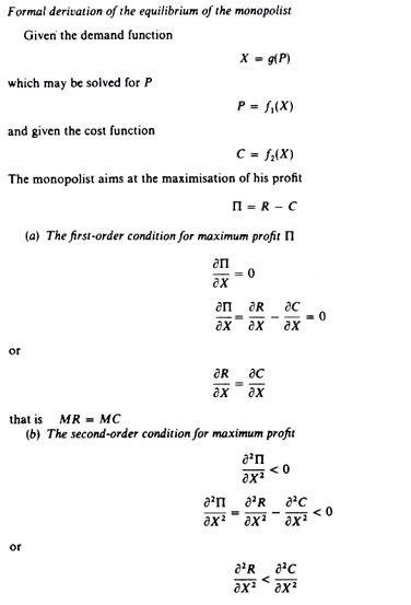
Monopoly price and output decision-equilibrium
A. Short run
A monopolist maximizes his short-term profits if the following two conditions are met first, MC equals Mr. Secondly; the slope of MC is larger than that of Mr at the intersection.
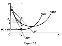
In Figure 6.2, the equilibrium of the monopoly is defined by the point θ at which MC intersects the MR curve from below. Thus, both conditions of equilibrium are met. The price is PM and the quantity is XM. Monopolies realize excess profits equal to shaded areas APM CB. Please note that the price is higher than Mr
In pure competition, the company is the one who receives the price, so it’s only decision is the output decision. The monopolist is faced with two decisions: to set his price and his output. But given the downward trend demand curve, the two decisions are interdependent.
Monopolies set their own prices and sell the amount the market takes on it, or produce an output defined by the intersection of MC and MR and are sold at the corresponding price. An important condition for maximizing the profits of monopolies is the equality of the MC and the MR, provided that the MC cuts the MR from below.
We can now revisit the statement that there is no unique supply curve for the monopolist derived from his MC. Given his MC, the same amount could be offered at different prices depending on the price elasticity of demand. This is graphically shown in Figure 6.3. Quantity X is sold at price P1 if demand is D1, and the same quantity X is sold at price P2 if demand is D2.
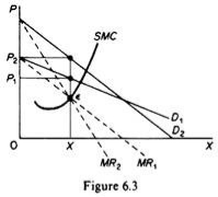
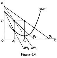
So there is no inherent relationship between price and quantity. Similarly, given the monopolist MC, we can supply various quantities at any one price, depending on the market demand and the corresponding MR curve. Figure 6.4 illustrates this situation. The cost condition is represented by the MC curve. Given the cost of a monopolist, he would supply 0X1 if the market demand is D1, then p at the same price, and only 0X2 if the market demand is D2 B.Long-term equilibrium:
In the long run the monopolist will have time to expand his plants or use his existing plants at every level to maximize his profits. However, if the entry is blocked, the monopolist does not need to reach the optimal scale (that is, the need to build the plant until the minimum point of LAC is reached), neither does the guarantee that he will use his existing plant at the optimum capacity. What is certain is that if he makes a loss in the long run, the monopolist will not stay in business.
He will probably continue to earn paranormal benefits even in the long run, given that entry is banned. But the size of his plant and the degree of utilization of any plant size depends entirely on the market demand. He may reach the optimal scale (the minimum point of Lac), stay on the less optimal scale (the falling part of his LAC), or exceed the optimal scale (expand beyond the minimum LAC), depending on market conditions.
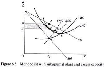
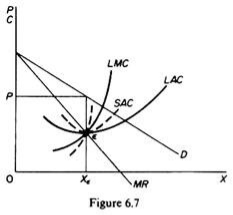
Figure 6.5 shows when the market size does not allow the monopolist to expand to the minimum point of Lac. In this case, not only is his plant not optimal (in the sense that the economy of full size is not depleted), but also the existing plant is not fully utilized. This is because on the left of the minimum point of the LAC, the SRAC touches the LAC at its falling part, and the short-term MC must be equal to the LRMC. This happens in e, but the minimum LAC is b,and the optimal use of the existing plant is a. Since it is utilized at Level E', there is excess capacity. Finally, figure 6.7 shows a case where the market size is large enough for a monopolist to build an optimal plant and be able to use it at full capacity.
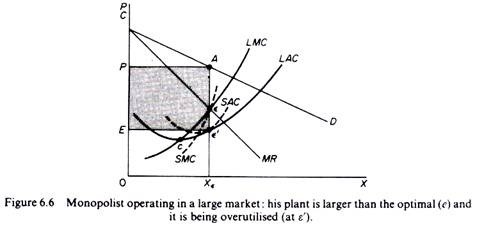
In Figure 6.6, the scale of the market is so large that monopolists have to build plants larger than the optimal ones to maximize output and over-exploit them. This is because to the right of the minimum point of LAC, SRAC and LAC is tangent at the point of positive slope, and SRMC must be equal to LAC. Thus, plants that maximize the profits of monopolies are, firstly, larger than the optimal size, and secondly, they are over-utilized, which leads to higher costs. This is often the case with utility companies operating at the state level.
It should be clear that which of the above situations will appear in a particular case will depend on the size of the market (given the technology of monopolists). There is no certainty that monopolies will reach their optimal size in the long run, as is the case with purely competitive markets. In Monopoly, there is no market force similar to those of pure competition that will lead companies to operate at optimal plant size in the long run (and utilize it at its full capacity).
Price determination
A monopolistic firm is a price-maker, not a price-taker. Therefore, a monopolist can increase or decrease the price. Also, when the price changes, the average revenue, and marginal revenue changes too. Take a look at the table below:
Quantity sold | Price per unit | Total revenue | Average revenue | Marginal revenue |
1 | 6 | 6 | 6 | 6 |
2 | 5 | 10 | 5 | 4 |
3 | 4 | 12 | 4 | 2 |
4 | 3 | 12 | 3 | 0 |
5 | 2 | 10 | 2 | -2 |
6 | 1 | 6 | 1 | -4 |
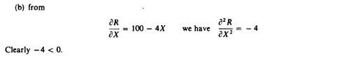
Let’s look at the revenue curves now:
As you can see in the figure above, both the revenue curves (Average Revenue and Marginal Revenue) are sloping downwards. This is because of the decrease in price. If a monopolist wants to increase his sales, then he must reduce the price of his product to induce:
Hence, the demand conditions for his product are different than those in a competitive market. In fact, the monopolist faces demand conditions similar to the industry as a whole.
Therefore, he faces a negatively sloped demand curve for his product. In the long-run, the demand curve can shift in its slope as well as location. Unfortunately, there is no theoretical basis for determining the direction and extent of this shift.
Talking about the cost of production, a monopolist faces similar conditions that a single firm faces in a competitive market. He is not the sole buyer of the inputs but only one of the many in the market. Therefore, he has no control over the prices of the inputs that he uses.
Role of time element in determination of price are given below:
Time plays an important role in the theory of volume, i.e., price determination because supply and demand conditions are affected by time.
Price during the short-period can be higher or lower than the cost of production, but in the long-period price will have a tendency to be equal to the cost of production.
The relative importance of supply on demand in the determination of price depends upon the time given to supply to adjust itself to demand.
To study the relative importance of supply or demand in price determination, Prof. Marshall has divided time element-into three categories:
(a) Very short period or market period.
(b) Short period.
(c) Long period.
(a) Very short period (determination of market price):
Market period is a time period which is too short to increase production of the commodity in response to an increase in demand. In this period the supply cannot be more than existing stock of the commodity.
The supply of perishable goods is perfectly inelastic during market period. But non-perishable goods (durable goods) can be stored.:
Therefore, the supply curve of non-perishable goods above reserve price has a positive scope at first but becomes perfectly inelastic after some price level.
The reserve price y depends upon-(i) cost of storing, (ii) future expected price, (iii) future cost of production, and (iv)seller’s need for cash we will discuss the determination of market price by taking a perishable commodity and determination of market price is illustrated.
DD is the original demand curve and SS the market period supply curve. The demand curve DD (perfectly inelastic) cuts the supply curve SS at point E. Point E, is the equilibrium point and equilibrium price is determined at OP, level.
Increase in demand shifts the demand curve to D,D and the price also increased to OP,. Decrease in demand shifts the demand curve downward to D2D2 and the price too falls to OP It is, thus, clear that in market period price fluctuates with change in demand conditions.
(b) Price determination is short period:
In the short period fixed factors of production remain unchanged, i.e., productive capacity remains unchanged.
However, in the short period supply can be affected by changing the quantity of variable factors.
In other words, during the short period supply can be increased to some extent only by an intensive use of the existing productive capacity.
Therefore, the supply curve in the short-run slopes positively, but the supply curve is less elastic. Determination of price in the short-run is illustrated.
SS is the market period supply curve and SRS is short-run supply curve. The original demand curve DD cuts both the supply curves at E, point and thus OP, price is determined.
Increase in demand shifts the demand curve upward to the right to D,D,. Now with the increase in demand the market price (in market period) rises at once to OP3 because supply remains fixed.But in the short-run supply increases. Therefore, in the short-run price will cuts the SRS curve. If demand decreases opposite will happen.
(c) Price determination in long period (Normal Price):
In the long period there is enough time for the supply to adjust fully to the changes in demand.
In the long period all factors are variable. Present firms can increase on decrease the size of their plants (productive capacity).
The new firms can enter the industry and old firms can leave the market. Therefore, long-period supply curve has a positive slope and is more elastic than short period supply curve.
The shape of supply curve of the industry depends upon the nature of the laws of returns applicable to the industry. Price determination in the long period is illustrated.
DD is the original demand curve and LS is the long period supply curve of the industry. Demand curve DD and supply curve LS both intersect each other at E point and OP price is determined.
This price will be equal to minimum average cost (AC) of production because in the long period firms under perfect competition can only earn normal profits. Suppose these are permanent increase in demand.
With the increase in demand, the demand curve shifts to D1,D1. As a result of increase in demand the price in the market period and short period will rise.
Due to increase in price present firms will earn above normal profit. Therefore, new firms will enter into market in the long period.
As a result of it supply will increase in the long period. In the long period price will be determined at OP1, level because at this price demand curve D1 D2 cuts the LS curve at E2 point.
Price OP1, is greater than previous price OP1, because the industry is an increasing cost industry. This new higher price will also be equal to minimum average cost of production
Monopolistic competition price and output decision-equilibrium
Under monopolistic competition a firm can some extent independently control the supply and price of the product. The demand curve is stable and slightly downward slope
A monopolistic competitor creates output at which the marginal cost is equal to marginal revenue. The price is greater than marginal cost.
Short run-
In short run, the firm attains its equilibrium where marginal revenue equals marginal cost and the price is set according to its demand curve. Thus when MR=MC, profits are maximized
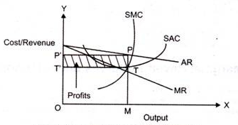
In the above fig,
AR is the average revenue curve,
MR represents the marginal revenue curve,
SAC curve represents the short run average cost curve,
SMC signifies the short run marginal cost.
In the above figure we can see that at output OM, MR intersects SMC. Here price is OP’ (which is equal to MP). Thus P is the point on AR curve, which is price. PT is the supper normal profit per unit output, is the difference between the average revenue and average cost.
Long run
In the long run due to the possibility of new firms entering the industry the price under monopolistic competition becomes equal to long-run average cost giving only normal profits. So, no firm under monopolistic competition can make excess profit or loss in the long run.
When the new firm start supplying , the price would fall. Thus the AR curve shifts from right to left and supernormal profits are replaced with normal profits. The long run equilibrium is achieved when average revenue is equal to average cost.
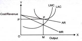
In the above fig we can see that, at pointP, AR curve touches the average cost curve (LAC) as a tangent. P is the equilibrium at price MP and output OM.
At MP average cost is equal to average revenue. Therefore, in long run, the profit is normal. The conditions (MR=MC and AR=AC) result in attaining equilibrium in long run.
Key takeaways –
Oligopoly
Oligopoly, in fact, describes the operation of a number of large corporations in the world. The operations of these markets are characterized by strategic behavior of a small number of rival firms. The extent of power as well as profits depends to a great extent on how rival firms react to each other’s decisions. If the behavior is less competitive, that is, if the rival firms behave in a cooperative manner, firms will enjoy market power and can charge prices above marginal cost.
An oligopolistic firm has to behave strategically when it makes a decision about its price. It has to consider whether rival firms will keep their prices and quantities constant, when it makes changes in its price and/or quantity. When an oligopolistic firm changes its price, its rival firms will retaliate or react and change their prices which in turn would affect the demand of the former ‑rm. Therefore, an oligopolistic firm cannot have sure and determinate demand curve, since the demand curve keeps shifting as the rivals change their prices in reaction to the price changes made by it. Now when an oligopolist does not know his demand curve, what price and output he will ‑x cannot be ascertained by economic analysis. However, economists have established a number of price-output models for oligopoly market depending upon the behaviour pattern of other firms in the market. Different oligopoly settings give rise to different optimal strategies and diverse outcomes. Important oligopoly models are:
Kinked demand model
In oligopolistic market, the competitors change the prices/quantity of output and thus firm cannot have a fixed demand curve. The price remain inflexible for a long time. American economist Sweezy in 1939 came up with the kinked demand curve to explain the behaviour of oligopolistic organizations.
A kinked demand curve occurs when the demand curve is not a straight line but due to higher and lower prices, it has a different elasticity ie elastic and inelastic.
Assumption of kinked demand curve model
The following figure shows a kinked demand curve dD with a kink at point P.
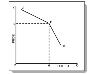
From the above fig, we can see that at price P, the firm produces and sell output at OM. the upper segment dP of the demand curve dD is elastic as the price rises the demand falls. The lower segment PD of the demand curve dD is relatively inelastic as the price falls, demand for the product increases.
This model suggest that price are rigid and with the increase or decrease in price the firm will face different affects. The kink in the demand curve is due to the behaviour of rival firms to the increase or decrease in price
Impact of price rise
Impact of price cut
Example of kinked demand curve
The market of petrol is homogenous and consumers are price sensitive. If one petrol pump increases the price, consumer will shift to other petrol station. If one petrol station will cut the price, the other station will also follow and cut the price.
Collusive oligopoly – price-leadership model
Collusion occurs when the rival firms agree to work together. They together set high price in order to make greater profits. Collusion refers to making higher profit in the expense of the consumer and reduces the competition in the market. Collusion is an agreement to seek higher price.
Definition
According to Samuelson, “Collusion denotes a situation in which two or more firms jointly set that prices or output, divide the market among them, or make other business decisions.”
In the words of Thomas J. Webster, “Collusion represents a formal agreement among firms in an oligopolistic industry to restrict competition to increase industry profits.”
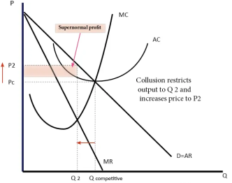
In the above figure we can see that when the industry is competitive quantity Q is given at price P1. As the firm collude, the price increase to P2 and quantity reduced to Q2. Thus the firm earns super normal profit.
Types of collusion
2. Tacit collusion – it is also referred as implicit collusion. This happens when two or more firms within the same industry informally agree to control the market.
3. Price leadership - Price leadership occurs when a firm leading in a given industry and can effectively determines the price of goods and services for the entire market. This type of firm is referred as price leaders. Price leadership is “situation in which a market leader sets the price of a product or services and competitors feel compelled to match that price”
Problems of collusion
Collusion is regulated by the government as it is seen bad for consumers and economic welfare. Collusion can lead to
Price leadership
Price leadership occurs when a firm leading in a given industry and can effectively determines the price of goods and services for the entire market. This type of firm is referred as price leaders.
Price leadership is “situation in which a market leader sets the price of a product or services and competitors feel compelled to match that price”
A dominant company sets the price and other firms with little choice have to follow its leads and adjust the price to match the price of the leading firm to hold their market share. Large firms commonly use price leadership as a strategy.
Effective leadership works under following conditions
Types of price leadership
There are three types of price leadership which includes barometric, collusive, and dominant.
a) In dominant price leadership, only one organisation dominates the entire industry.
b) It is also referred as partial monopoly.
c) Under this the leading firm sets the prices and the smaller firms providing same products and services adjust and match the price of the leading firm.
d) The dominant firm use its monopoly power to maximise the profits.
e) The dominant firm ignores the interest of other organisation.
f) The price leader follows predatory pricing, which refers to lowering prices to levels so that smaller, competing firms find difficulty to remain in business.
2. Barometric –
a) Under barometric, one organisation at first declares the change in the price and assumes that other organisation will accept it.
b) The organisation need not to be leader of the firm and does not dominate others.
c) Barometric leader have less power to impose its decision on the other firms.
d) Organisation which lacks capacity to estimate appropriate supply and demand conditions they follow the price changes made by barometric leaders.
e) Barometric leader is preferred as one organisation is not the only leader.
3. Collusive
a) Collusive leadership is an agreement between the dominant firms to keep their prices in mutual alignment.
b) This type of leadership is used in industry where the entry cost is high and cost of production is known.
c) Smaller firms follow the price change effectively.
d) It is done to avoid competition.
e) This involves illegal agreement to disrupt the market equilibrium and gain unfair market advantage.
f) The firm collude to avoid uncertainties and maximise the joint profit.
Duopoly
Duopoly is a limiting case of oligopoly, in the sense that it has all the characteristics of oligopoly except the number of sellers which are only two increase of duopoly as against a few in oligopoly. The main distinguishing feature of duopoly (and also of oligopoly) from other market situating is that the sellers’ decisions are not independent of each other. A change in price and output by our seller affect the former, and now the former may have to react. This process of action- reaction of the sellers may continue. This when a duopolist (or an oligopolist) takes any policy decision he also takes into account the reactions of his rivals. That is, such a market situation is characteristics by the mutual interdependence in policy-making.
There are various types of duopoly models pertaining to price-output decisions under duopoly market situation
a) a French economist Augustin Cournot was the first to develop a formal duopoly model in 1838.
b) This model is implied when firm produces homogenous goods, they compete simultaneously on market share and output, they expect any changes the firm make, in response the rivals not to change their output.
c) Cournot uses the example of mineral spring water. Both the firm operates at zero marginal cost. The demand curve face constant negative slope. Each seller acts on the assumption that his competitor will not react to his decision to change his and price.
d) The model conclude that each firm supplies one-third of the market and charges the same price. While one-third of the market remains unsupplied.
e) The model is criticised that the assumption zero cost of production is totally unrealistic
2. Chamberlin’s duopoly model
a) Chambrilin states that the firm takes into account the reaction of other firms to the firms output and price decision.
b) His model is based on assumption of homogeneous products, firms of equal size with identical costs, no entry by new firms and full knowledge of demand.
c) The single oligopolistic takes into account both the direct as well as the indirect effects of his decisions.
d) Each oligopolist must be aware of the marginal costs of other firms.
e) According to chamberlin, the recognition of reaction to an oligopolistic firms price and output decision would avert harmful competition and would result in a stable industry equilibrium with the monopoly price and monopoly output.
3. Bertrand’s Duopoly Model
a) A French Mathematician Bertrand, developed his own model of duopoly in 1883.
b) On the basis of behavioural assumption Bertrand’s model differs from Cournot’s model.
c) Cournot assumes rival output remains constant. While under Bertrand’s model seller determines his price on the assumption that rivals price remains constant.
d) This model focuses on price competition.
e) The firm thinks by marginally cutting the price with others price remain same, it can capture the entire market.
f) The other firm also respond and price war flares up.
g) The process of cutting the price to capture the market goes on as long as the price exceeds the marginal cost of the firm at its current sales.
4. Stakelberg’s duopoly
a) Under this model, each seller from his experience becomes aware of this rival reaction to his sales plan.
b) The firm then estimates his rival’s reaction curve and then make his own calculation to choose a profit maximising output.
c) A firm allows his rival’s reaction in its decision making is called a leader by Stackelberg.
5. Sweezy’s Kinked Demand Model:
a) American economist Sweezy in 1939 came up with the kinked demand curve to explain the behaviour of oligopolistic organizations.
b) A kinked demand curve occurs when the demand curve is not a straight line but due to higher and lower prices, it has a different elasticity ie elastic and inelastic.
Non price competition
Non-price competition involves ways that firms seek to increase sales and attract custom through methods other than price. Non-price competition can include quality of the product, unique selling point, superior location and after-sales service.
Non-Price competition in Oligopoly/imperfect competition
The majority of industries are a form of oligopoly with a few firms dominating the market. The firms in an oligopoly can compete in price, but often non-price competition becomes the most important factor dominating the market.
The kinked demand curve model suggests that in oligopoly prices will be stable – leading to firms concentrating on non-price competition.
In monopolistic competition, there is freedom of entry, but firms have a degree of market power (inelastic demand curve) because of product differentiation. Therefore, firms in monopolistic competition have a motive to try and improve their product differentiation and brand image.
Price discrimination and product differentiation
Price discrimination It is a situation when a monopolist charges different prices from different buyers of the same product. This is generally done to maximise profits, e.g. in a monopoly, surgeon in your area may charge low fee from the poor patients and high fee from the rich patients.
Product differentiation It is a situation when different producers under monopolistic competition try to differentiate their product in terms of its shape, size, packing, trademark or brand name. This is done to attract buyers from the rival firms in the market.
Key takeaways –
Sources-


