UNIT-2
Distributions
A random variable whose value cannot be arranged in a sequence, is called continuous random variable.
Continuous random variable is represented by different representation, called probability density function.
Probability density function-
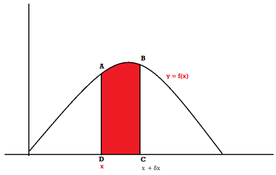
Suppose f(x) be a continuous function of x . Suppose the shaded region ABCDshown in the following figure represents the area bounded by y = f( x ), x –axis and the ordinates at the points x and x + δx , where δx is the length of the interval ( x , x + δx ).if δx is very-very small, then the curve AB will act as a line and hence the shaded region will be a rectangle whose area will be AD × DCthis area = probability that X lies in the interval ( x, x +δx )
= P[ x≤ X ≤ x +δx ]
Hence,


Properties of Probability density function-
1. 
2. 
Example: If a continuous random variable X has the following probability density function:

Then find-
1. P [0.2 < X < 0.5]
Solution:
Here f(x) is the probability density function, then-


A function F defined for all values of a random variable X by
F( x ) = P[X ≤ x ] is called the distribution function. It is also known as the cumulative distribution function (c.d.f.) of X since it is the cumulative probability of X up to and including the value x.
Continuous Distribution Function
Distribution function of a continuous random variable is called the continuous distribution function or cumulative distribution function (c.d.f.).
Let X be a continuous random variable having the probability density function
f( x ), as defined in the last section of this unit, then the distribution function
F( x ) is given by

Example: The pdf of a continuous random variable is given as below-

Then find the c.d.f. Of X.
Solution:
The c.d.f. Of X will be given by-


Hence the c.d.f will be-


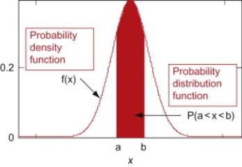
Probability density function (PDF) is a arithmetical appearance which gives a probability distribution for a discrete random variable as opposite to a continuous random variable. The difference among a discrete random variable is that we check an exact value of the variable. Like, the value for the variable, a stock worth, only goes two decimal points outside the decimal (Example 32.22), while a continuous variable have an countless number of values (Example 32.22564879…).
When the PDF is graphically characterized, the area under the curve will show the interval in which the variable will decline. The total area in this interval of the graph equals the probability of a discrete random variable happening. More exactly, since the absolute prospect of a continuous random variable taking on any exact value is zero owing to the endless set of possible values existing, the value of a PDF can be used to determine the likelihood of a random variable dropping within a exact range of values.
Distribution Function:
Let X be a D.R.V. Then its discrete distribution function or cumulative distribution function (c.d.f.) is defined as –

Exponential Distribution:
The exponential distribution is a C.D. Which is usually use to define to come time till some precise event happens. Like, the amount of time until a storm or other unsafe weather event occurs follows an exponential distribution law.
The one-parameter exponential distribution of the probability density function PDF is defined:
f(x)=λ ,x≥0,
,x≥0,
Where, the rate λ signifies the normal amount of events in single time.
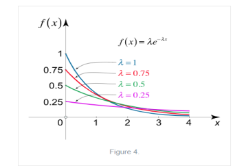
The mean value is μ= . The median of the exponential distribution is m =
 , and the variance is shown by
  .
.
Normal Distribution:
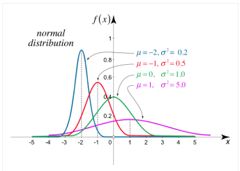
The normal distribution is the utmost broadly identified P.D. Then it defines many usual spectacles.
The PDF of the normal distribution is shown by method
f(x) =  ,
,
Where μ is mean of the distribution, and  is the variance.
The 2 limitations μ and σ completely describe the figure and all additional things of the normal distribution function.
Gamma density
Consider the distribution of the sum of 2 autonomous Exponential ( ) R.V.
Density of the form:

Density is knowm Gamma (2, density. In common the gamma density is precise with 2 reasons (t,
 as being non zero on the +ve reals and called:

Where  is the endless which symbols integral of the density quantity to one:

By integration by parts we presented the significant recurrence relative:

Because , we have for integer t=m

The specific case of the integer t can be linked to the sum of n independent exponential, it is the waiting time to the nth event, it is the matching of the negative binomial.
From that we can estimate what the estimated value and the variance are going to be: If all the Xi's are independent exponential ( , then if we sum n of them we
Have  and if they are independent:
This simplifies to the non-integer t case:

Example1: Following probability distribution
x | 0 | 1 | 2 | 3 | 4 | 5 | 6 | 7 |
P(x) | 0 |  |  |  |  |  |  |  |
Find: (i) k (ii) 
(i) Distribution function
(ii) If  find minimum value of C
(iii) Find 
Solution:
If P(x) is p.m.f –


(i)
X | 0 | 1 | 2 | 3 | 4 | 5 | 6 | 7 |
P(x) | 0 |  |  |  |  |  |  |  |
(ii)


(iii)
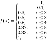
(iv)


(v)


B: Bivariate Distributions
Bivariate discrete random variables-
Let X and Y be two discrete random variables defined on thesample space S of a random experiment then the function (X, Y) defined onthe same sample space is called a two-dimensional discrete random variable. Inothers words, (X, Y) is a two-dimensional random variable if the possiblevalues of (X, Y) are finite or countably infinite. Here, each value of X and Y isrepresented as a point ( x, y ) in the xy-plane.
Joint probability mass function-
Let (X, Y) be two-dimensional discrete random variables with each possible outcome  , we associate a number
  representing-

And satisfying the given conditions-

The function p defined for all  is called joint probability mass function of X and Y.
Conditional probability mass function-
Let (X, Y) be a discrete two-dimensional random variable. Then the conditional probability mass function of X, given Y = y is defined as-


Because-

A bivariate distribution, setonly, is the probability that a definite event will happen when there are 2 independent random variables in your scenario. E.g, having two bowls, individually complete with 2dissimilarkinds of candies, and drawing one candy from each bowl gives you 2 independent random variables, the 2dissimilar candies. Since you are pulling one candy from each bowl at the same time, you have a bivariate distribution when calculating your probability of finish up with specific types of candies.
Properties:
Property 1
Two random variable X and V are said to be bivariate normal, or jointly normal, if aX +bY has a normal distribution for all a, 
Properties 2:
Two random variable X and V are said to be standard bivariate normal distribution with correlation coefficient  if their joint PDF is given by

Where  . If
. If  , then we just say X and Y have the standard bivirate normal distribution.
Properties 3:
Two random variable X and V are said to be bivariate normal distribution with parameters  if their joint PDF is given by


Where,  and
and  are all constants
Properties 4:
Suppose X and Y are jointly variables with parameters  . Then given X=x,Y is normally distributed with


Example 1:
Let  be two independent N(0,1) random variables. Define


Where  is a real number in (-1,1)
a. Show that X and Y are bivariate normal.
b. Find the joint PDF of X and Y.
c. Find  (X,Y)
(X,Y)
Solution:
First, note that since  are normal and independent, they are jointly normal with the joint PDF


We need to show aX+bY is normal for all  we have


 and thus it is normal.
 We can use the methods of transformations (Theorem 5.1) to find the joint PDF of X and Y. The inverse transformation is given by


Thus we conclude that,


 To find
  , first mode


Therefore,


Example 2:
Let X and Y be jointly normal random variables with parameters  Find the conditional distribution of Y given X =x.
Solution:

One way to solve this problem is by using the joint PDF formula since X N
N  we can use


Thus given X=x, we have

And,

Since  are independent, knowing
  does not provide any information on
  . We have shown that given X=x,Y is a linear function of
  , thus it is normal. Ln particular


We conclude that given X=x,Y is normally distributed with mean  and variance
Example 3;
Let X and Y be jointly normal random variables with parameters 
(a) Find 
(b) Find 
(c) Find 
Solution:
(a)Since X and Y are jointly normal, the random variable V-2X+Y is normal. We have


Thus,  , therefore,

(b)Note that 


(c)Using Properties, we conclude that given X=2,Y is normally distributed with


Thus,

Given random variables X and Y that are defined on a probability space, the joint probability distribution for X and Y is a probability distribution that gives the probability that each of X and Y falls in any particular range or discrete set of values specified for that variable. In the case of only two random variables, this is called a bivariate distribution, but the concept generalizes to any number of random variables, giving a multivariate distribution.
The joint probability distribution can be expressed either in terms of a joint cumulative distribution function or in terms of a joint probability density function (in the case of continuous variables) or joint probability mass function (in the case of discrete variables). These in turn can be used to find two other types of distributions: the marginal distribution giving the probabilities for any one of the variables with no reference to any specific ranges of values for the other variables, and the conditional probability distribution giving the probabilities for any subset of the variables conditional on particular values of the remaining variables.
Example - A die is tossed thrice. A success is getting 1 or 6 on a toss. Find the mean and variance of the number of successes.
Solution:
Probability of mean success =
Probability of failures=
Probability of no success =Probability of all 3 failures =
Probability of one success and 2 failures
Probability of two success and one failure
Probability of three successes 
Now,
 0 1 2 3
 =8/27 4/9 2/9 1/27
Mean,

Also,
Variance,
Example-The probability density function of a variate X is
X 0 1 2 3 4 5 6
P(X) k 3k 5k 7k 9k 11k 13k
(i) Find 
(ii) What will be the minimum value of k so that  .
.
Solution:
(i) If X is a random variable, then


(ii) 
Thus minimum value of k 
Example- A random variable X has the following probability function
x: 0 1 2 3 4 5 6 7
p(x) 0 k 2k 2k 3k 
(i) Find the value of k.
(ii) Evaluate 
(iii) 
Solution:
(i) If X is a random variable then

i.e. 
(ii) 


(iii)

Let A and B are two event in a sample space S and P(B)≠0. Then the probability that an event A occurs once B has occurred or the conditional probability of A given B which is defined as-

Note- If two events A and B are independent then-

Multiplication theorem for conditional probability-

Example: A bag contains 12 pens of which 4 are defective. Three pens are picked at random from the bag one after the other.
Then find the probability that all three are non-defective.
Solution:
Here the probability of the first which will be non-defective = 8/12
By the multiplication theorem of probability,
If we draw pens one after the other then the required probability will be-

Example: The probability of A hits the target is 1 / 4 and the probability that B hits the target is 2/ 5. If both shoot the target then find the probability that at least one of them hits the target.
Solution:
Here it is given that-

Now we have to find- 
Both two events are independent. So that-


Bayes rule-
Let  and
and  be mutually exclusive events forming a portion of the sample space S and let E be any event of the sample space such that P(E) ≠ 0.
Then-
The Bayes theorem can be defined as-

Example: An urn I contains 3 white and 4 red balls and an urn II contains 5 white and6 red balls. One ball is drawn at random from one of the urns and is found to be white.
Find the probability that it was drawn from urn I.
Solution:
Let


Now we have to find-

So that by using Bayes theorem, we get-

Here,
Two urns are equally likely to select,


So that-

Example: In a bolt factory, machines A, B and C manufacture respectively 25%, 35% and 40% of the total. If their output 5, 4 and 2 per cent are defective bolts. A bolt is drawn at random from the product and is found to be defective. What is the probability that it was manufactured by machine B?
Solution:
Here-
A: bolt is manufactured by machine A
B: bolt is manufactured by machine B
C: bolt is manufactured by machine C
So that- P(A) = 0.25, P(B) = 0.35 and P(C) = 0.40
The probability of drawing a defective bolt manufactured by machine A is P(D/A) = 0.05
P (D/B) = 0.04 and P (D/C) = 0.02
Therefore by using Bayes theorem-

