UNIT-3
Basic statistics
Professor Bowley defines the average as-
“Statistical constants which enable us to comprehend in a single effort the significance of the whole”
An average is a single value which is the best representative for a given data set.
Measures of central tendency show the tendency of some central values around which data tend to cluster.
The following are the various measures of central tendency-
1. Arithmetic mean
2. Median
3. Mode
4. Weighted mean
5. Geometric mean
6. Harmonic mean
Arithmetic mean or mean-
Arithmetic mean is a value which is the sum of all observation divided by total number of observations of the given data set.
If there are n numbers in a dataset-  then arithmetic mean will be-

If the numbers along with frequencies are given then mean can be defined as-

Example-1: Find the mean of 26, 15, 29, 36, 35, 30, 14, 21, 25 .
Solution:


Example-2: Find the mean of the following dataset.
x | 20 | 30 | 40 |
f | 5 | 6 | 4 |
Solution:
We have the following table-
x | f | Fx |
20 | 5 | 100 |
30 | 6 | 180 |
40 | 7 | 160 |
| Sum = 15 | Sum = 440 |
Then Mean will be-


Direct method to find mean-
Example: Find the arithmetic mean of the following dataset-

Solution:
We have the following distribution-
Class interval | Mid value (x) | Frequency (f) | Fx |
0-10 | 05 | 3 | 15 |
10-20 | 15 | 5 | 75 |
20-30 | 25 | 7 | 175 |
30-40 | 35 | 9 | 315 |
40-50 | 45 | 4 | 180 |
|
| Sum = 28 | Sum = 760 |

Short cut method to find mean-
Suppose ‘a’ is assumed mean, and ‘d’ is the deviation of the variate x form a, then-

Example: Find the arithmetic mean of the following dataset.
Class | 0-10 | 10-20 | 20-30 | 30-40 | 40-50 |
Frequency | 7 | 8 | 20 | 10 | 5 |
Solution:
Let the assumed mean (a) = 25,
Class | Mid-value | Frequency | x – 25 = d | Fd |
0-10 | 5 | 7 | -20 | -140 |
10-20 | 15 | 8 | -10 | -80 |
20-30 | 25 | 20 | 0 | 0 |
30-40 | 35 | 10 | 10 | 100 |
40-50 | 45 | 5 | 20 | 100 |
Total |
| 50 |
| -20 |

Step deviation method for mean-

Where
Median-
Median is the mid value of the given data when it is arranged in ascending or descending order.
1. If the total number of values in data set is odd then median is the value of  item.
item.
Note-The data should be arranged in ascending r descending order
2. If the total number of values in data set is even then median is the mean of the  item.
item.
Example: Find the median of the data given below-
7, 8, 9, 3, 4, 10
Sol.
Arrange the data in ascending order-
3, 4, 7, 8, 9, 10
So there total 6 (even) observations, then-


=
Median for grouped data-

Here,


Example: Find the median of the following dataset-

Sol.
Class interval | Frequency | Cumulative frequency |
0 - 10 | 3 | 3 |
10 – 20 | 5 | 8 |
20 – 30 | 7 | 15 |
30 – 40 | 9 | 24 |
40 – 50 | 4 | 28 |

So that median class is 20-30.
Now putting the values in the formula-


So that the median is 28.57
Mode-
A value in the data which is most frequent is known as mode.
Example: Find the mode of the following data points-

Solution:
Here 6 has the highest frequency, so that the mode is 6.
Mode for grouped data-

Here,


Example: Find the mode of the following dataset-

Solution:
Class interval | Frequency |
0 - 10 | 3 |
10 – 20 | 5 |
20 – 30 | 7 |
30 – 40 | 9 |
40 – 50 | 4 |
Here highest frequency is 9. So that the modal class is 40-50,
Put the values in the given data-


Hence the mode is 42.86
Note-
Mean – Mode = [Mean - Median]
Geometric Mean-
If  are the values of the data, then the geometric mean-

Harmonic mean-
Harmonic mean is the reciprocal of the arithmetic mean-
It can be defined as-

Note-
1. 
2. 
Moments-
The r’th moment of a variable x about the mean is denoted by  and defined as-

The r’th moment of a variable x about any point ‘a’ will be-

Relationship between moments about mean and moment about any point-

Skewness-
The word skewness means lack of symmetry-
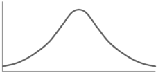
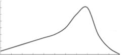
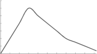
The examples of symmetric curve, positively skewd and negatively skewd curves are given as follows-
1. Symmetric curve-
2. Positively skewd-
3. Negatively skewd-
To measure the skewness we use Karl Pearson’s coefficient of skewness.
Then formula is as follows-

Note- the value of Karl Pearson’s coefficient of skewness lies between -1 to +1.
Kurtosis-
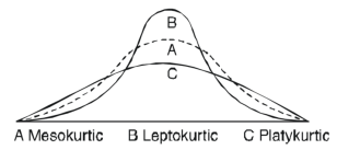
It is the measurement of the degree of peakedess of a distribution
Kurtosis is measured as-
Calculation of kurtosis-
The second and fourth central moments are used to measure kurtosis.
We use Karl Pearson’s formula to calculate kurtosis-

Now, three conditions arises-
1. If  , then the curve is mesokurtic.
2. If  , then the curve is platykurtic
3. If  , then the curve is said to be leptokurtic.
Example: If coefficient of skewness is 0.64. Standard deviation is 13 and mean is 59.2, then find the mode and median.
Solution:
We know that-

So that-


And we also know that-


Example: Calculate the Karl Pearson’s coefficient of skewness of marks obtained by 150 students.

Solution:
Mode is not well defined so that first we calculate mean and median-
Class | f | x | CF |  | Fd |  |
0-10 | 10 | 5 | 10 | -3 | -30 | 90 |
10-20 | 40 | 15 | 50 | -2 | -80 | 160 |
20-30 | 20 | 25 | 70 | -1 | -20 | 20 |
30-40 | 0 | 35 | 70 | 0 | 0 | 0 |
40-50 | 10 | 45 | 80 | 1 | 10 | 10 |
50-60 | 40 | 55 | 120 | 2 | 80 | 160 |
60-70 | 16 | 65 | 136 | 3 | 48 | 144 |
70-80 | 14 | 75 | 150 | 4 | 56 | 244 |
Now,


And

Standard deviation-

Then-


Where-
1. 
2. 
The set of values  with their probabilities
  constitute a discrete probability distribution of the discrete variable X.
Binomial distribution-
A discrete random variable X is said to be follow the binomial distribution with parameter n and p.
The probability of happening of an event r times exactly in n trials is-

Example: A die is thrown 8 times then find the probability that 3 will show-
1. Exactly 2 times
2. At least 7 times
3. At least once
Solution:
As we know that-


Then-
1. Probability of getting 3 exactly 2 times will be-

2. Probability of getting 3 at least 7 or 8 times will be-

3. Probability of getting 3 at least once or (1 or 2 or 3 or 4 or 5 or 6 or 7 or 8 times)-


Example: If the percentage of failure in a test is 20. If six students appear in the test, then what will be the probability that at least five students will pass the test?
Solution:
Here


Then the probability of at least five students will pass the test-


Mean and standard deviation of binomial distribution-
1. 
2. 
3. 
Moments of binomial distribution-
1. First moment about the origin-

2. Second moment about the origin-

3. Third moment about origin-

4. Fourth moment about origin-

5. Third central moment-

6. Fourth central moment-

Example: Find mean and variance of a binomial distribution with p = 1/4 and n = 10.
Solution:
Here 
Mean = np = 
Variance = npq = 
Example: If a dice is rolled thrice. A success is getting 1 or 6 on a roll. Find the mean variance of the number of success.
Solution:
Here n = 3 , p = 1/3 and q = 2/3
Mean = np = 1
And variance = npq = 2/3
Poisson distribution-
Poisson distribution is a limiting case of binomial distribution under certain conditions listed below-
1. n, the number of trials are infinitely large.
2. p, the probability of success for each trial is very small.
3. Np is finite quantity say 
A random variable X is said to be follow Poisson distribution if it has the following probability mass function-


Moments of Poisson distribution-
1. First moment about origin-  which Is known as mean.
2. Second moment about origin- 
3. Third moment about origin- 
4. Fourth moment about origin- 
Note-
1. Poisson distribution is always positively skewed distribution.
2. Mean and variance of Poisson dist. Are always equal
For Poisson distribution-


Example: If cars arriving at workshop follow the Poisson distribution. If the average number of cars arrivals during a specified period of an hour is 2.
Find the probabilities that during the given hour-
1. No car arrive
2. At least two cars arrive.
Solution:
Here the average of car arrivals is - 2
So that mean = 2

Let X be the number of cars arriving during the given hour,
By using Poisson distribution, we get-

So that the required probability-
1. P [no car will arrive] = P [X = x] = 
2. P [At least two cars will arrive] = P [X≥2] = P [X =2] + P [X = 3] + ……….
= 1 - P [[X =1] + P [X =0]]


Example: If the probability that a vaccine given to the patients shows bad reaction is 0.001, then find the probability that out of 2000 patients-
1. Exactly 3 patients
2. More than 2 patients
3. No patient
Will show bad reaction.
Solution:
Here p = 0.001 and number of patients (n) = 2000
Then 
By using Poisson distribution, we get-

1. Probability that exactly 3 patients show bad reaction is-

2. Probability that more than 2 patients show bad reaction-


3. Probability that no patient shows bad reaction-

Example: If a book has 600 pages and it has 40 printing mistakes. Assume that these mistakes are randomly distributed and x the number of mistakes per page follow Poisson distribution.
What is the probability that there will not be any mistake if 10 pages selected at random?
Solution:
Here 
We get by using Poisson distribytion-

Then-

Normal Distribution-
The concept of normal distribution was given by English mathematician Abraham De Moivre in 1733 but the concrete theory was given by Karl Gauss that is why sometime normal distribution is called Gaussian distribution.
Normal distribution is a continuous distribution. It is a limiting case of binomial distribution.
The probability density function of a normal distribution is given by-

Here 
Where 
Note-
1. If a random variable X follows normal distribution with mean  and variance
  then we can write it as- X
2. If X  , then
  is called standard normal variate with mean 0 and standard deviation 1.
3. The probability density function of standard normal variate Z is given as-

Where 
Graph of a normal probability function-
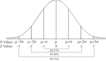
The curve look like bell-shaped curve. The top of the bell is exactly above the mean.
If the value of standard deviation is large then curve tends to flatten out and for small standard deviation it has sharp peak.
This is one of the most important probability distributions in statistical analysis.
Example:
1. If X  then find the probability density function of X.
2. If X  then find the probability density function of X.
Solution:
1. We are given X 
Here 
We know that-

Then the p.d.f. will be-

2. . We are given X 
Here 
We know that-

Then the p.d.f. will be-

Mean median and mode of the normal distribution
Let ‘a’ is the median, then it divides the total area into two parts-

Where-

Let a>mean, then-
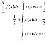
Thus-

So that mean = median.
Note- mean deviation about mean is = 
Mode-
The mode of the normal distribution is  and modal ordinate is given by-

Hence the mean, median and mode are equal in normal distribution.
Area property of a normal distribution (Area under the normal curve)-
Let X follows the normal distribution with mean  and variance
We form a normal curve by taking 
Note- Total area under the curve is always 1.
Example: If a random variable X is normally distributed with mean 80 and standard deviation 5, then find-
1. P[X > 95]
2. P[X < 72]
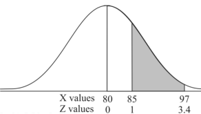
3. P [85 < X <97]
[Note- use the table- area under the normal curve]
Solution:
The standard normal variate is – 
Now-
1. X = 95,

So that-


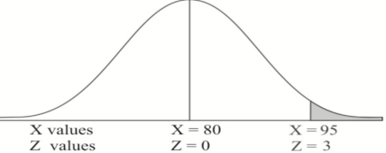
2. X = 72,

So that-


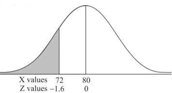
3. X = 85,

X = 97,

So that-


Example: In a company the mean weight of 1000 employees is 60kg and standard deviation is 16kg.
Find the number of employees having their weights-
1. Less than 55kg.
2. More than 70kg.
3. Between 45kg and 65kg.
Solution:
Suppose X be a normal variate = the weight of employees.
Here mean 60kg and S.D. = 16kg
X 
Then we know that-

We get from the data,

Now-
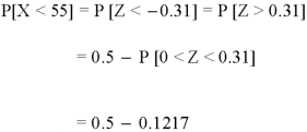
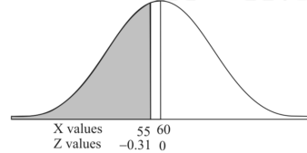
1. For X = 55,

So that-

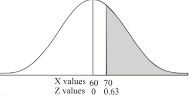
2. For X = 70,

So that-


3. For X = 45,

For X = 65,


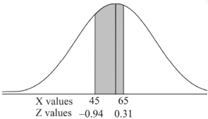
Hence the number of employees having weights between 45kg and 65kg-

Example: The mean inside diameter of a sample of 200 washers produced by a machine is 0.0502 cm and the standard deviation is 0.005 cm. The purpose for which these washers are intended allows a maximum tolerance in the diameter of 0.496 to 0.508 cm, otherwise the washers are considered defective. Determine the percentage of defective washers produced by the machine, assuming the diameters are normally distributed.
Solution:
Here-

And

Area for non-defective washers = area between z = -1.2 to +1.2
= 2 area between z = 0 and z = 1.2
= 2 × 0.3849 = 0.7698 = 76.98%
Then percent of defective washers = 100 – 76.98 = 23.02 %
Example: The life of electric bulbs is normally distributed with mean 8 months and standard deviation 2 months.
If 5000 electric bulbs are issued how many bulbs should be expected to need replacement after 12 months?
[Given that P (z ≥ 2) = 0. 0228]
Solution:
Here mean (μ) = 8 and standard deviation = 2
Number of bulbs = 5000
Total months (X) = 12
We know that-

Area (z ≥ 2) = 0.0228
Number of electric bulbs whose life is more than 12 months ( Z> 12)
= 5000 × 0.0228 = 114
Therefore replacement after 12 months = 5000 – 114 = 4886 electric bulbs.
When two variables are related in such a way that change in the value of one variable affects the value of the other variable, then these two variables are said to be correlated and there is correlation between two variables.
Example- Height and weight of the persons of a group.
The correlation is said to be perfect correlation if two variables vary in such a way that their ratio is constant always.
Scatter diagram-
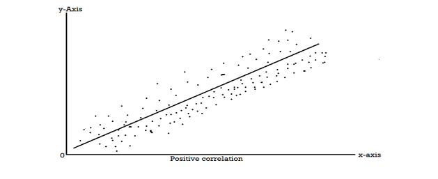
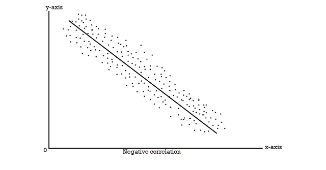
Karl Pearson’s coefficient of correlation-

Here-  and
and 

Note-
1. Correlation coefficient always lies between -1 and +1.
2. Correlation coefficient is independent of change of origin and scale.
3. If the two variables are independent then correlation coefficient between them is zero.
Correlation coefficient | Type of correlation |
+1 | Perfect positive correlation |
-1 | Perfect negative correlation |
0.25 | Weak positive correlation |
0.75 | Strong positive correlation |
-0.25 | Weak negative correlation |
-0.75 | Strong negative correlation |
0 | No correlation |
Example: Find the correlation coefficient between Age and weight of the following data-
Age | 30 | 44 | 45 | 43 | 34 | 44 |
Weight | 56 | 55 | 60 | 64 | 62 | 63 |
Solution:
x | y |  |  |  |  | (   |
30 | 56 | -10 | 100 | -4 | 16 | 40 |
44 | 55 | 4 | 16 | -5 | 25 | -20 |
45 | 60 | 5 | 25 | 0 | 0 | 0 |
43 | 64 | 3 | 9 | 4 | 16 | 12 |
34 | 62 | -6 | 36 | 2 | 4 | -12 |
44 | 63 | 4 | 16 | 3 | 9 | 12 |
Sum= 240 |
360 |
0 |
202 |
0 |
70
|
32 |
Karl Pearson’s coefficient of correlation-

Here the correlation coefficient is 0.27.which is the positive correlation (weak positive correlation), this indicates that the as age increases, the weight also increase.
Short-cut method to calculate correlation coefficient-

Here,


Example: Find the correlation coefficient between the values X and Y of the dataset given below by using short-cut method-
X | 10 | 20 | 30 | 40 | 50 |
Y | 90 | 85 | 80 | 60 | 45 |
Solution:
X | Y |  |  |  |  |  |
10 | 90 | -20 | 400 | 20 | 400 | -400 |
20 | 85 | -10 | 100 | 15 | 225 | -150 |
30 | 80 | 0 | 0 | 10 | 100 | 0 |
40 | 60 | 10 | 100 | -10 | 100 | -100 |
50 | 45 | 20 | 400 | -25 | 625 | -500 |
Sum = 150 |
360 |
0 |
1000 |
10 |
1450 |
-1150 |
Short-cut method to calculate correlation coefficient-


Spearman’s rank correlation-
When the ranks are given instead of the scores, then we use Spearman’s rank correlation to find out the correlation between the variables.
Spearman’s rank correlation coefficient can be defined as-

Example: Compute the Spearman’s rank correlation coefficient of the dataset given below-
Person | A | B | C | D | E | F | G | H | I | J |
Rank in test-1 | 9 | 10 | 6 | 5 | 7 | 2 | 4 | 8 | 1 | 3 |
Rank in test-2 | 1 | 2 | 3 | 4 | 5 | 6 | 7 | 8 | 9 | 10 |
Solution:
Person | Rank in test-1 | Rank in test-2 | d =  |  |
A | 9 | 1 | 8 | 64 |
B | 10 | 2 | 8 | 64 |
C | 6 | 3 | 3 | 9 |
D | 5 | 4 | 1 | 1 |
E | 7 | 5 | 2 | 4 |
F | 2 | 6 | -4 | 16 |
G | 4 | 7 | -3 | 9 |
H | 8 | 8 | 0 | 0 |
I | 1 | 9 | -8 | 64 |
J | 3 | 10 | -7 | 49 |
Sum |
|
|
| 280 |


Regression-
Regression is the measure of average relationship between independent and dependent variable
Regression can be used for two or more than two variables.
There are two types of variables in regression analysis.
1. Independent variable
2. Dependent variable
The variable which is used for prediction is called independent variable.
It is known as predictor or regressor.
The variable whose value is predicted by independent variable is called dependent variable or regressed or explained variable.
The scatter diagram shows relationship between independent and dependent variable, then the scatter diagram will be more or less concentrated round a curve, which is called the curve of regression.
When we find the curve as a straight line then it is known as line of regression and the regression is called linear regression.
Note- regression line is the best fit line which expresses the average relation between variables.
Equation of the line of regression-
Let
y = a + bx ………….. (1)
Is the equation of the line of y on x.
Let  be the estimated value of
  for the given value of
  .
.
So that, According to the principle of least squares, we have the determined ‘a’ and ‘b’ so that the sum of squares of deviations of observed values of y from expected values of y,
That means-

Or
 …….. (2)
Is minimum.
Form the concept of maxima and minima, we partially differentiate U with respect to ‘a’ and ‘b’ and equate to zero.
Which means


And


These equations (3) and (4) are known as normal equation for straight line.
Now divide equation (3) by n, we get-

This indicates that the regression line of y on x passes through the point .
.
We know that-

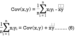
The variance of variable x can be expressed as-


Dividing equation (4) by n, we get-

From the equation (6), (7) and (8)-

Multiply (5) by , we get-

Subtracting equation (10) from equation (9), we get-


Since ‘b’ is the slope of the line of regression y on x and the line of regression passes through the point ( ), so that the equation of the line of regression of y on x is-


This is known as regression line of y on x.
Note-
 are the coefficients of regression.
2. 
Example: Two variables X and Y are given in the dataset below, find the two lines of regression.
x | 65 | 66 | 67 | 67 | 68 | 69 | 70 | 71 |
y | 66 | 68 | 65 | 69 | 74 | 73 | 72 | 70 |
Solution:
The two lines of regression can be expressed as-

And

x | y |  |  | Xy |
65 | 66 | 4225 | 4356 | 4290 |
66 | 68 | 4356 | 4624 | 4488 |
67 | 65 | 4489 | 4225 | 4355 |
67 | 69 | 4489 | 4761 | 4623 |
68 | 74 | 4624 | 5476 | 5032 |
69 | 73 | 4761 | 5329 | 5037 |
70 | 72 | 4900 | 5184 | 5040 |
71 | 70 | 5041 | 4900 | 4970 |
Sum = 543 | 557 | 36885 | 38855 | 37835 |
Now-

And

Standard deviation of x-


Similarly-


Correlation coefficient-


Put these values in regression line equation, we get
Regression line y on x-


Regression line x on y-


Regression line can also be find by the following method-
Example: Find the regression line of y on x for the given dataset.
X | 4.3 | 4.5 | 5.9 | 5.6 | 6.1 | 5.2 | 3.8 | 2.1 |
Y | 12.6 | 12.1 | 11.6 | 11.8 | 11.4 | 11.8 | 13.2 | 14.1 |
Solution:
Let y = a + bx is the line of regression of y on x, where ‘a’ and ‘b’ are given as-


We will make the following table-
x | y | Xy |  |
4.3 | 12.6 | 54.18 | 18.49 |
4.5 | 12.1 | 54.45 | 20.25 |
5.9 | 11.6 | 68.44 | 34.81 |
5.6 | 11.8 | 66.08 | 31.36 |
6.1 | 11.4 | 69.54 | 37.21 |
5.2 | 11.8 | 61.36 | 27.04 |
3.8 | 13.2 | 50.16 | 14.44 |
2.1 | 14.1 | 29.61 | 4.41 |
Sum = 37.5 | 98.6 | 453.82 | 188.01 |
Using the above equations we get-


On solving these both equations, we get-
a = 15.49 and b = -0.675
So that the regression line is –
y = 15.49 – 0.675x
Note – Standard error of predictions can be find by the formula given below-

Difference between regression and correlation-
1. Correlation is the linear relationship between two variables while regression is the average relationship between two or more variables.
2. There are only limited applications of correlation as it gives the strength of linear relationship while the regression is to predict the value of the dependent varibale for the given values of independent variables.
3. Correlation does not consider dependent and independent variables while regression consider one dependent variable and other indpendent variables.
B: Applied statistics
Method of least square-
Suppose
y = a + bx ………. (1)
Is the straight line has to be fitted for the data points given-

Let  be the theoretical value for
Now-


For the minimum value of S -

Or

Now

Or

On solving equation (1) and (2), we get-


These two equations are known as the normal equations.
Now on solving these two equations we get the values of a and b.
Example: Find the straight line that best fits of the following data by using method of least square.
X | 1 | 2 | 3 | 4 | 5 |
y | 14 | 27 | 40 | 55 | 68 |
Solution:
Suppose the straight line
y = a + bx…….. (1)
Fits the best-
Then-
x | y | Xy |  |
1 | 14 | 14 | 1 |
2 | 27 | 54 | 4 |
3 | 40 | 120 | 9 |
4 | 55 | 220 | 16 |
5 | 68 | 340 | 25 |
Sum = 15 | 204 | 748 | 55 |
Normal equations are-


Put the values from the table, we get two normal equations-


On solving the above equations, we get-

So that the best fit line will be- (on putting the values of a and b in equation (1))

To fit the second degree parabola-

The normal equations will be-

Note- Change of scale-
We change the scale if the data is large and given in equal interval.
As-

Example: Fit the second degree parabola of the following data by using method of least squares.
X | 1929 | 1930 | 1931 | 1932 | 1933 | 1934 | 1935 | 1936 | 1937 |
Y | 352 | 356 | 357 | 358 | 360 | 361 | 361 | 360 | 359 |
Solution:
By taking u = x – 1933 and v = y – 357
Then equation  becomes
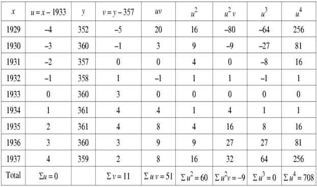
Putting the values from the table in normal equations-
We get-
11 = 3A + 0B + 60C or 11 = 9A + 60C
51 = 0A + 60B + 0C or B = 17 / 20
-9 = 60A + 0B + 708C or -9 = 60A + 708C
On solving, we get-


On solving the above equation, we get-

Example: Fit the curve  by using the method of least square.
X | 1 | 2 | 3 | 4 | 5 | 6 |
Y | 7.209 | 5.265 | 3.846 | 2.809 | 2.052 | 1.499 |
Solution:
Here-


Now put-
Then we get-

x | Y |  | XY |  |
1 | 7.209 | 1.97533 | 1.97533 | 1 |
2 | 5.265 | 1.66108 | 3.32216 | 4 |
3 | 3.846 | 1.34703 | 4.04109 | 9 |
4 | 2.809 | 1.03283 | 4.13132 | 16 |
5 | 2.052 | 0.71881 | 3.59405 | 25 |
6 | 1.499 | 0.40480 | 2.4288 | 36 |
Sum = 21 |
| 7.13988 | 19.49275 | 91 |
Normal equations are-

Putting the values form the table, we get-
7.13988 = 6c + 21b
19.49275 = 21c + 91b
On solving, we get-
b = -0.3141 and c = 2.28933
c = 
Now put these values in equations (1), we get-
