Unit 8 | unit 8 turbulent flow

Unit - 8

Turbulent Flow

8.1 Reynolds Experiment

The process of conducting laboratory research to find out the significant number of Reynolds pipe flow in various discharge cases is described in this article.

Reynolds number is the ratio of the unbalanced energy of a liquid to the energy of a viscous fluid. Non-liquid energy can be expressed by:

Inertia force, Fi = mass × acceleration

= (density × volume) X (Velocity / time)

= (density X Area) X (Velocity X Velocity)

F I = A V 2

Viscous strength, Fv = Shear stress X area

F v = v D

Therefore, Reynolds' number is provided by:

R e = F I / F v = A V 2 / v D = rho v D / = v D /

Where, v = velocity of flow fluid

D = width of glass metal

Apparatus required

Water tank

A small pond filled with colored liquid or dye

A glass tube with a bell mouth door

Measurement tank

Control valve in glass shop and dye injector entry

Stopwatch

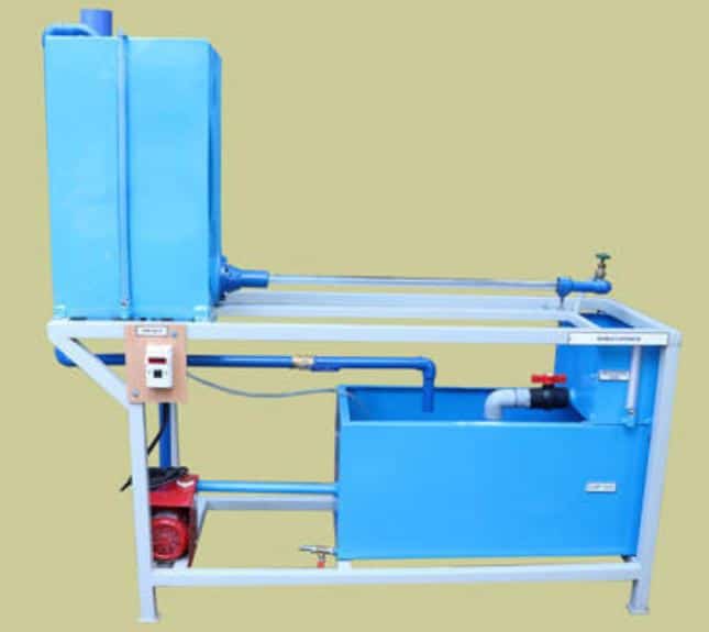
Fig no 1 Reynolds experiment apparatus

Test Process

The Reynolds test process is as follows:

Fill the tank with water and leave it for a while as the water in the tank should rest.

Now fill the reservoir with a dye (usually a solution of potassium permanganate) that is nothing but colored liquid. The weight of the dye should be equal to water.

Record water temperature.

Allow glass flow to flow at a much lower level by slightly opening the glass tube exit valve.

When the flow is stable, open the dye injection valve and allow the colored liquid to flow through the glass tube.

Reynolds Resources Applicable Performance

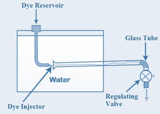
Fig no 2 Operational Status of Reynolds Resources

Look at the appearance of the dye plate in the glass tube and write down the type of flow found in that extract.

Take a stopwatch and write down the amount of water collected to measure a certain time period.

Repeat the above procedure for different output values and calculate the Reynolds number for each flow type.

Calculation

The volume of water collected in a tank in t seconds, V = tank area X Water level in t seconds

Release, Q = Volume / time

Velocity of flow, v = Extrusion / location of glass tube

Reynolds number, Re =

Example:

Q.1 A pipeline carrying water has average height of irregularities projecting from the surface of the boundary of the pipe as 0.12 mm. What type of boundary is it? The shear stress developed is 4.9 N/m2. The kinematic viscosity of water is 0.01 strokes.

Solution:

Given

Height of irregularities k= 0.15 mm

Shear stress

Kinematic viscosity

Density of water

Step 1 Shear stress

Step 2 Roughness Reynolds’s number

Since Re > 4 but less than 100 the surface is transition

Q.2 For turbulent flow through a pipe having wall shear stress 10 N/m², size of surface imperfection is k = 0.03 mm. Assuming the kinematic viscosity of water 1 x 10 m³/sec. find whether pipe behave as hydro dynamically rough, smooth or transitional.

Soln.:

Given: Shear stress = 10 N/m²

Size of surface imperfection k= 0.03 mm = 0.03 x 10³ m

Kinematic viscosity v = 1x10 m²/sec.

Density of water = 1000 kg/m³

Step 1: Shear stress,

Step 2: Roughness Reynolds’s number,

Re= 0.03 < 4

Since less than 4, between 4 and 100, and hence pipe Since surface behaves as smooth.

Q.3 A pipe line carrying oil s= 0.8 has average height of irregularities projecting from the surface of the boundary of the pipe as 0.3 mm. What type of boundary is it? The shear stress developed is 3N/m². Take kinematic viscosity v = 0,012 stoke.

Soln.:

Given:

Average height of irregularities K = 0.3 mm = 0.3 x 10³ m

Shear stress =3 N/mm²

Specific gravity of oil s=0.8.

Density p=800 kg-m¹

Kinematic viscosity v=0.012 stoke=0.012x 10 m²/sec.

Step 1: Shear stress,

Step 2: Roughness Reynolds’s number,

15.25> 4 but <100

The surface boundary is transition.

Q.4 Air (p = 1.22 kg/m³ and v = 1.5 x 10 m³/s) flows through 250 mm diameter pipe at 8 m/s as mean velocity. If the equivalent sand grain roughness is 0.5 mm, calculate wall shear stress and friction factor f. Assume flow to be fully rough turbulent and neglect compressibility.

Soln.:

Given: p = 1.22 kg/m²

v = 1.5x 10³ m²/sec.

d = 250 mm = 0.25 m.

R= 0.125 m, u = 8 m/sec.,

K = 0.5 mm = 5 x 10¹ m

Step 1: Reynolds’s number

The flow is turbulent in the rough pipe.

Step 2: For rough turbulent pipe

Step 3: Shear stress at the pipe surface

The wall shear stress is 0.134 N/m² and friction factor is 0.0137.

Key takeaways

The process of conducting laboratory research to find out the significant number of Reynolds pipe flow in various discharge cases is described in this article.

Reynolds number is the ratio of the unbalanced energy of a liquid to the energy of a viscous fluid

8.2 Transition from Laminar to Turbulent Flow

At fluid dynamics, the process of laminar flow becomes chaotic known as laminar-turbulent transformation. The largest parameter showing the change is Reynolds number.

Transformation is often described as a process that goes on in a series of stages. "Temporary flow" may refer to a change in any direction, that is a temporary or volatile flow.

This procedure applies to any fluid flow, and is widely used in the context of boundary layers.

Transition stages in boundary layers

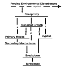
Fig no 3 The path from receptivity to laminar turbulent transition

The boundary layer can change into chaos in many ways. Which path is physically visible depends on the initial conditions such as the initial height of the disturbance and the size of the area. The level of understanding of each phase varies greatly, from a complete understanding of the development of the basic mode to a complete penetration of the understanding of the transit patterns.

Receptivity

The first phase of the evolutionary process is known as the Acceptance phase and consists of the conversion of natural disturbances - both acoustic (noise) and vertical (turbulence) - into minor disturbances within the boundary layer.

The mechanisms by which these disturbances occur vary and include free stream noise and / or turbulence associated with local curvature, vertical position and magnitude. These initial conditions are small, often irreversibly disrupted by the basic state flow.

From here, the growth (or decay) of this disorder depends on the nature of the disorder and the type of basic state. Acoustic disturbances often favor two-dimensional instability such as Toll mien- Schlichting waves (TS waves), while vertical disturbances often lead to the development of three-dimensional conditions such as crossing instability.

Numerous experiments in recent decades have shown that the size of the enlargement region, which is why the area where the surface changes in the body, strongly depends not only on the size and / or width of the external disturbance but also on their physical condition. Some interference easily penetrates the boundary layer while others do not.

As a result, the concept of transition of the boundary layer is complex and lacks a complete definition of doctrine.

Primary mode growth

If the initial disruption, caused by nature is small enough, the next stage of the transformation process is the growth of the first mode. At this stage, the initial disruption grows (or decays) in the manner described by the concept of stable stability.

Some identified defects are actually dependent on the geometry of the problem and the nature and severity of the initial disturbance. Throughout the Reynolds numerical range in a given flow configuration, the greatly enhanced modes can vary and are often different.

There are many major types of instability that occur frequently across border crossings. In subsonic flow and pre-supersonic onset, large two-dimensional forces with TS waves. In the flow where a three-dimensional layer rises like a swept wing, the instability of the road flow becomes significant.

In the rotating surface of the concave surface, Gortler's vortices can be a major instability. Each instability has its own body base and its own control strategies - some of which are opposed to other instability - which add to the difficulty of controlling turbulent change.

Simple harmonic boundary layer sound in the physics of transition to turbulence

The simple harmonic sound as a deterrent to the sudden conversion from laminar to turbulent flow can be attributed to Elizabeth Barrett Browning. His poem, Aurora Leigh (1856), explores how musical notes (the identification of a particular church bell), begin to rumble through the flames of street lights ("... lights tremble in the streets and squares": Hair 2016).

His soon-to-be-praised poem may have warned scientists (e.g., Leconte 1859) of the influence of light harmonic sound (SH) as a cause of turmoil. The modern advancement of scientific interest in this came to the fore in Sir John Tyndall (1867) who determined that certain SH sounds, directed directly at the flow, had waves interacting with the same SH waves created by collisions at the boundaries of the tubes, enlarging them and causing miraculous disruption. His definition appeared more than 100 years later (Hamilton 2015).

Toll mien (1931) and Schlichting (1929) suggest that the viscosity along the smooth border, creates oscillations of the SH boundary layer (BL) that gradually increase in amplitude until a disturbance arises.

Although the wind tunnels of the day failed to substantiate this theory, Schubauer and Skramstad (1943) built a tunnel of pure air that calmed the vibrations and the sounds that could impede the air tunnel lessons of the flow of plates.

They have confirmed the long-term improvement of BL heating, the shear waves of shifting shear switching. They have shown that special SH vibrations induced electromagnetically into the BL ferromagnetic ribbon can amplify the same wavelengths introduced by SH BL flutter (BLF), reducing turbulence at very low flow rates. In addition, certain wavelengths interfere with the growth of SH BLF waves, keeping the laminar flow to high flow rates.

The release of weight from a liquid is a vibration that creates a sound wave. The burning of the SH BLF in the liquid of the line layer next to the flat plate should produce a SH sound indicating the boundary corresponding to the liquid laminae.

In the late transition, Schubauer and Skramstad have found the focus of increasing BL oscillations, which is accompanied by explosion ("disturbed areas"). Focused expansion of the dynamic sound over time is associated with the formation of the BL vortex.

The intensified noise of the turbulent areas next to a flat plate with the potential for striking molecules in contrast to the laminar, may suddenly cause slippery local ice. Sudden collapse of "frozen" spots can transmit high resistance at the border, and may explain the head-over-heels vortices of BL vortices of late late. Osborne Reynolds described areas of similar turmoil during the transition of cylinder water flow (“light of turbulence,” 1883).

When multiple random vortices explode as chaos erupts, the normal cooling of the laminar slide (connected connection) is associated with noise and a significant increase in flow resistance.

This may also explain the is velocity profile of the dynamic laminar flow that suddenly changes to the blurred profile of the turbulent flow - as the laminar slip is replaced by a laminar connection as the turbulence arises (Hamilton 2015).

Second instability

The main mechanisms themselves do not directly lead to deterioration, but instead lead to the formation of secondary instability mechanisms.

As the main methods grow and distort the flow you mean, they begin to show inconsistencies and the straightforward concept no longer works.

What makes the problem worse is the growing distortion of the flow you mean, which can lead to points from the acceleration profile of the situation shown by Lord Rayleigh to show complete instability at the boundary.

This second instability quickly leads to deterioration. This second instability is often much higher than their previous grades.

Examples:

Q.1 Determine the wall shearing stress in a pipe of diameter 100 mm which carries water. The velocities at the pipe centre and 30 mm from the pipe centre are 2 m/s and 1.5 m/s respectively. The flow in pipe is given as turbulent.

Soln.:

Given:

Diameter, D = 100 mm = 0.1 m,

Radius, R = 50 mm = 0.05 m

Velocity of centre, U = 2 m/sec

Velocity of 30 mm from centre u = 1.5 m/s,

y = 0.05-0.03 = 0.02 m

For turbulent flow,

Wall shear stress,

Q.2 In a pipe of diameter 150 mm, carrying water the velocities at the pipe centre and 45 mm from pipe centre are found to be 2.5 m/s and 2 m/s respectively. Find the wall shearing stress.

Soln.:

Given: Diameter of pipe D = 150 mm = 0.15m,

:. Radius R = 0.15/2 = 0.075 m 2

Velocity of centre U=2.5 m/s,

Velocity at 45mm

U = 2 m/sec

At u = 2 m/sec, y = 0.075 -0.045 = 0.03 m

For turbulent Velocity

Shear stress,

Q.3 In a pipe of diameter 100 mm carrying water, the velocities at the pipe centre and 20 mm from the pipe centre are found to be 2.5 ms and 2.3 m/s respectively. Find the wall shear stress.

Soln.:

Given: D-100 mm-0.1m,

Radius R=005 m.

Velocity at centre U=2.5 m/s,

Velocity at 20 mm

u=2.3 m/s,

Velocity 2.3 m/s from pipe wall, y=0.05-0.02 -0.03m

For Turbulent flow

Shear stress

Q.4 In a smooth pipe of diameter 0.5 m and length 900 m, water is flowing at a rate of 0.05 m/sec. Assuming kinematic viscosity of water as 0.02 stokes, find:

(1) Head lost due to friction

(2) Centre line velocity sub layer.

(3) Wall shear stress

(4) Thickness of laminar

Take friction factor f= 0.314/(Re)^(1/4) for turbulent.

Soln.:

Given:

d=0.5 m.

L=900 m. Q=0.05 m/sec.

V= 0.02 stokes.

Step 1: Mean velocity,

Step 2: Reynolds’s number,

Step 3: The flow is turbulent,

Step 4: Head loss by Darcy-Weisbach equation,

Step 5: Wall shear stress,

Step 6: Shear velocity.

Step 7: For turbulent flow in smooth pipe, maximum velocity is,

For y=-=0.25 m, v = (1.e. centre line viscosity)

Step 8: Thickness of laminar sub-layer

Q.5 An oil with a kinematic viscosity 0.2 stoke and specific weight diameter is 30 cm and the discharge is 0.1 m/s. Determine 8000 N/m flows through a pipe. The pipe is smooth and its the maximum velocity through the pipe, thickness of the laminar sub layer, boundary shear stress and the velocity at the edge of the laminar sub layer.

Soln.:

Given: v= 0.2 stoke=0.2 x 10 m/Sec=8000 N/m,

D= 30cm=0.3 m, Q = 0.1 m'/Sec

To find: Umax,

Mean velocity, u= Q/A =0.1/0236 = 0.4244 m/s

Reynolds number Re= ud/v= 0.4244x0.3/ 0.2x10

= 6366.19 >4000

As the Reynolds number is more than 4000, the flow is turbulent Friction factor by blasius equation

Shear velocity,

Maximum velocity for turbulent flow n smooth pipe is = 5.75 1080 (+55

for y = D/2=3=0.15m,

Thickness of laminar sub-layer

Velocity at the edge of laminar sub-layer, y = 8

Q.6 For turbulent flow through a pipe 60 cm in diameter, the velocities are 4.5 m/s and 4.2 m/s on the centre line and at a radial distance of 10 cm from pipe axis. Calculate the discharge in the pipe.

Soln.:

Given: D = 60 cm = 0.6 m, R = 0.3 m

Velocity at centre U=4.5 m/s.

Velocity at r=0.1 m, u = 4.2 m/s

Distance from wall surface y R-r-03-0.1-0.2 m

For turbulent flow

Relation between mean velocity and average velocity

Discharge Q

Q.7 A fluid with specific gravity 1.1 and kinematic viscosity 1 x 10 m/s is to be pumped through a smooth pipe of diameter 300 mm over a length of 1 km. Flow rate is 4 m/min Calculate minimum pressure and power rating of the pump.

Soln.

Given=

S= 11, v=1x10 m/h,

L= 1 km =1000 m

d = 300 mm = 0,3 m, Q = 4 m/min = 0.0667 m²/sec

Step 1: Velocity.

Step 2: Reynolds’s number,

The flow is turbulent, Assume pipe is to be smooth.

Step 3: Nikuradse's empirical formula, when 10¹<R,<4x10'

Step 4: Head loss due to friction,

Step 5: Minimum pressure,

Step 6: Power rating of the pump,

Key takeaways

At fluid dynamics, the process of laminar flow becomes chaotic known as laminar-turbulent transformation. The largest parameter showing the change is Reynolds number.

Transformation is often described as a process that goes on in a series of stages. "Temporary flow" may refer to a change in any direction, that is a temporary or volatile flow.

8.3 Definition of Turbulence

Turbulence is one of the most unpredictable of all the weather phenomena that are of significance to pilots.

Turbulence is an irregular motion of the air resulting from eddies and vertical currents. It may be as insignificant as a few annoying bumps or severe enough to momentarily throw an airplane out of control or to cause structural damage.

Turbulence is associated with fronts, wind shear, thunderstorms, etc.

Key takeaways

Turbulence is one of the most unpredictable of all the weather phenomena that are of significance to pilots.

8.4 Scale and Intensity

In reporting a disturbance, it is often considered light, moderate, severe or extreme. The level is determined by the type of initial agency and the level of air stability.

Light turbulence

A slight turbulence temporarily causes a slight change in height and / or attitude or a slight explosion. Airplane occupants may feel overwhelmed when faced with their seat belts.

Moderate

The moderate chaos is similar to a small chaos but more intense. However, there is no loss of flight control. Employees will experience obvious difficulties in their seat belts and unprotected items will be released.

Severe turbulence

Severe turmoil creates a dramatic and sudden change in altitude and / or attitude, and, more often than not, a significant variation in the airspeed shown. The flight may be temporarily out of control. The crew will be forced to violently fasten their seat belts.

Extreme turbulence

In the worst case scenario, the plane is thrown violently and it is impossible to control it. It can cause structural damage.

Chop is a type of disorder that causes a rapid and rhythmic eruption

Key takeaways

There are different scale and intensity of turbulence like

light

moderate

serve turbulence

extreme turbulence

8.5 Causes of Turbulence

There are four causes of unrest.

1. Mechanical turbulence

Conflicts between air and soil, especially unfamiliar terrain and man-made barriers, cause eddy and therefore turbulence at lower levels. The intensity of this confusing movement depends on the strength of the atmosphere, the atmosphere and the stability of the air. The stronger the wind speed (usually, more than 20 or more knots are needed for a major disturbance), the worse the environment and the more unstable the wind, the more chaos there will be. Of all the factors that contribute to the formation of chaos, stability is the most important.

When the air is heated from below, the vertical movement will be much stronger and wider and the stiffness is more noticeable. In unstable winds, eddys tend to grow in size; in stable conditions, they usually do not grow in size but are slightly scattered.

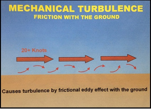
Fig no 4 Mechanical turbulence

In strong winds, even hangar and large structures cause eddy to move some distance from the ground. Strong winds often become stronger; that is, they change rapidly at speed. A sudden increase in speed that lasts for several minutes is known as squalls and they face a very serious turmoil.

Stagnant mountain eddies are found down in the mountains. They are caused and therefore stand in the face of mountain slopes. The mountain waves produce some of the most complex disturbances associated with mechanical organizations. NOTE: The stability of the lower troposphere above and to the mountain is very important (i.e., the most intense turbulence is associated with a stable upper airline and the appearance of a mountain barrier).

Favorable mountain wave conditions include:

Wind 25 knots or more, striking differently on top of a mountain.

Slight change in wind direction with length

Increased wind speed

Stable condition (should be cold air

Crossing over or over the mountain, a layer of low stability near the earth, a very stable layer at the top of the mountain above the upper layer, and finally, the unstable layer over the unstable layer) -

This requires air parcels to be forced to rise above the mountain peaks to sink at their first elevation (or at the level of equilibrium)

The parcels then get up and fall into the oscillatory pattern, similar to a heavy spring

Frequency from the face upwards tropopause

It can extend 100 miles or more downstream mountains

Main refurbishment and downdraft wave can remove a plane up to 5,000 feet per minute.

Construction projects can be stretched over the mountain side

The strongest turbulence is found in the lowlands, south of the mountains in or near the rotor cloud, if any

Mountain waves can be represented by clouds of mountain waves -

Cirrocumulus Standing Lenticular (CCSL)
Altocumulus Standing Lenticular (ACSL) closely related
Rotor Clouds (tense frequency)

2. Thermal turbulence

Anarchy can also be expected on a hot summer day when the sun heats the earth unevenly. Some areas, such as barren land, rocky outcrops, and soils, are heated much faster than grass-covered fields and much faster than water.

The separating currents therefore begin with the movement of warm air and cool air, which is subjected to extreme conditions as the plane enters and exits. Chaos from the base to the top of the convection layer, with the smooth conditions found above.

if cumulus, long cumulus or cumulonimbus clouds are present, the turbulent layer extends from the top to the tops of the clouds.

Turbulence power increases as the transmission pressure exceeds. In hot weather where most work is not expected, many pilots prefer to fly early in the morning or in the evening when the hot work is not as intense.

The parallel currents may not be made visible by cumuliform clouds, leading to "dry thermals". Favorite conditions of dry convection include higher temperatures, uneven local sensitivity, and high-end ground-based temperatures.

Transmission currents are usually strong enough to produce thunderstorms accompanied by high turbulence. Confusion can also be expected at low levels of cold air that travels over a warm area. Heat from below creates unstable conditions, strong winds, and extreme flying conditions.

The hot turmoil will have a significant impact on the flight path of the destination. The plane is under the transmission currents of various forces moving across the earth near the approach. These thermals can remove a plane from its normal glide path with the effect that it will override or pull down the path.

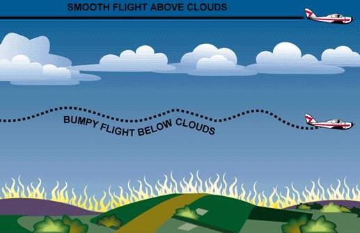
Fig no 5 Thermal turbulence

3. Frontal turbulence

The rising air temperature in the front slope and the friction between these opposing wind bodies create tension in the front area. This disorder is most pronounced when warm air is moist and unstable and will be more severe when thunderstorms occur. Confusion is often associated with colder climates but can be, to a lesser extent, warmer.

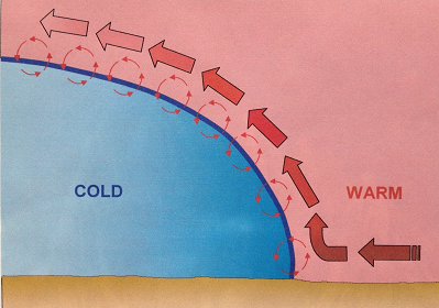
Fig no 6 Frontal turbulence

4. Wind shear

Wind shear changes in wind direction and / or wind speed over a specific or precise distance. Climatic conditions in which there is a shear of air include: temperature change zones, tunnels and basements, and jet distribution. When changing the wind speed and direction, a very turbulent storm can be expected. Clear air turbulence associated with very high altitudes (i.e., over 15,000 meters AGL) and jet propulsion.

Temperature changes are the strongest areas for air shaving. Strong stability prevents the combination of a stable lower layer with a warmer surface. The largest shear, and thus the largest turmoil, is found at the tops of the conversion layer. The turbulence associated with temperature changes often occurs as a result of cooling, which cools the earth's surface at night, resulting in surface-based inversion.

The turbulence associated with the lower pillars and rhinos is due to direct cutting and speed cutting. The turbulence is found in mounds at any height, within the fall at any height, and in the lowest and middle and lowest rows.

Jet propulsion is the backbone of strong horizontal winds following a wave-like pattern as part of the overall air flow. It is found where there is a large horizontal difference in temperature between the warm and cold air masses. The turmoil is located in the solid isotach gradient. Typically, chaos is found on the opposite side of the cyclonic jet. On the other hand, chaos is often found on the equator side of the anti cyclonic jet river. The turbulence is enhanced by the "arching" (amplified) jet stream around the rhinos and hills.

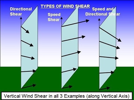
Fig no 7 Wind shear

Key takeaways

There are mainly 4 types of causes for turbulence

mechanical

thermal

frontal

wind

8.6 Instability

Liquid instability is evident everywhere in nature. The flow of fluid will begin in the laminar and is smooth and then progress quickly to the wrong pattern and eventually to the chaos.

The only thing you have to do is to see its increase in the sky looking on a cloudy day when the conditions are right as there will be big clouds passing by each other and growing designs.

This is Kelvin-Helmholtz instability (where there is a shear between two liquids with different speeds).

Another common instability when adding cold milk to hot tea. The amount of cold moisture falls and removes the hot water, and it is clear that certain structures are forming.

The same situation occurs in the flow of contents, such as pipes, or in infinite flow, such as that above the wing or without a tap.

In all of these cases, the simplest solution can lead to the solution of our unconscious view of the unpredictable world, where the fluid retains its smooth structure, but this does not happen.

Instead, the specific size and shape of the structures of the structure, usually occurs from time to time, and the structure grows until it becomes very turbulent until the flow is no longer a long laminar, but has turned into chaos.

Normal mode analysis can usually be performed (when it is assumed that the motion statistics are in a form where different wavelengths can be tested), and by solving the equation, a growth rate of different wavelengths is obtained.

This will tell us what configuration is expected. When new engineering devices incorporate fluid flow, it is important to respond to these issues.

This can be to try and reduce the onset of the disorder (or acceleration) or to understand the length of the various waves that can create and may cause resonance or unwanted behavior.

Key takeaways

Liquid instability is evident everywhere in nature. The flow of fluid will begin in the laminar and is smooth and then progress quickly to the wrong pattern and eventually to the chaos.

The only thing you have to do is to see its increase in the sky looking on a cloudy day when the conditions are right as there will be big clouds passing by each other and growing designs.

8.7 Mechanism of Turbulence and Effect of Turbulent Flow in Pipes

Mechanism of Turbulence

The turbulence machine works in conjunction with the capillary gate mechanism. It describes the nature of high blood pressure, pulpable pulse, atherosclerosis, and arterial thrombosis. The key to understanding hemodynamic physiology is a non-Newtonian blood type, which eliminates confusion during rapid systolic blood flow.

The red cell “binds” the form automatically during acceleration of systolic blood pressure and eliminates systolic inflammation, so that the heart releases its contents through excessive activity.

The expandable vein tree expands to accommodate the increased volume. At the end of the systole, the heart relaxes and blood flow briefly changes direction to the aorta to close the aortic valve.

The narrowed width of the distal aorta exaggerates the flow of fluid, disrupts the composite structure, and initiates the explosion of a fast-moving tumor throughout the artery tree, slowing down the flow of movement as it travels.

The tumor prevents atherosclerosis and thrombosis, and creates side effects that describe blood pressure. Behind the pulse wave, the pulmonary artery acts as a “second heart” that facilitates laminar blood flow in capillary beds, but is too small to be measured by normal metals.

The lateral force is a force that explains blood pressure is clearly altered by several factors including vessel width, length, separation and stiffness; body temperature; and blood viscosity (flow resistance).

Mammalian physiology maintains body temperature above the limit of lipoprotein liquefaction to prevent lipoprotein binding which increases blood viscosity. Opening the capillary port reduces blood viscosity, improves tissue absorption, and lowers blood pressure, such as normal sleep.

Closing the capillary port increases blood viscosity, reduces tissue absorption, and increases blood pressure. Blood pressure is therefore a contradictory and ineffective method of medical management.

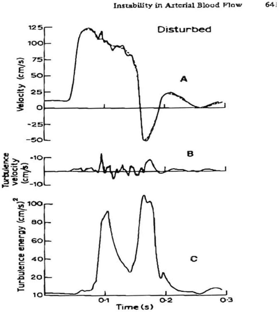
Fig no 8 Mechanism graph of turbulence

Aortic disturbance in the dog. Blood speeds from 0 to 100 cm / second and the heart beats less than one tenth of a second. Simultaneous systolic flow of Mammalian prevents atherosclerosis and improves flow efficiency, muscle relaxation, tissue oxygenation, and exercise tolerance.

Effect of Turbulent Flow in Pipe

Interaction Effect

Turbulence in turbine phases depends on many aerodynamic aspects and flow conditions. In this chapter, the author attempts to shed light, based on previously researched activities, on nonlinear effects and methods of electrical losses, on how they rely on the effects of chaos and how aerodynamic performance can be disrupted.

In a comprehensive review of loss-generating methods for the turbo machinery was introduced. The three main sources of loss in the turbine phase, are defined as: shear viscous in boundary layers, shear layers and mixing processes; process such as shock waves and heat transfer processes.

Boundary layers are known as the best looking regions, and can be referred to as areas of velocity gradients and shear pressures. In the boundary line, a higher amount of energy loss is produced in areas where dense gradients are found.

In a parameter called the “coefficient” Cd is defined. Its variability in laminar and turbulent boundary layer layers, and Reynolds numbers in the range of 300 <Reθ<1000, indicates that the predictive nature of the change is very important in the loss test in turbomachinery boundary lines.

Stator and rotor blades intersect, So unstable flow disturbances will occur in both vertical and rotating frames. Various aerodynamic effects, such as blood flow to the next edge, second flow in the radial direction, metal movement, flow in axial spaces, shock waves and effects in subsequent transitions in transonic phases, attack angles at the leading edges, etc., can greatly affect rotor blades and their efficiency. Load blades and power, working with blades, are much lower under the conditions mentioned above, resulting in less performance.

Condensation Effect

Condensation processes in turbo machines are random and unstable. The rate of droplet growth indicates a variety of factors, known as numerical comparisons and tests, also measured by real low-pressure turbines. This difference is due to a sharp decrease in temperature, which is caused by the separation of blade wakes (especially those at the edges of the track) by successive rows of blades.

In the case of a two-phase flow, one must specify the consequences of the disturbance in relation to the gas and water phases. In other words, gas phase disturbances can be affected in two ways including the dispersed phase and droplet movement can also be influenced by chaos.

Part of the fluid velocity measurement will affect the normal flow of flow particles. Two identical particles can have different energies due to the specificity of air flow, such as secondary flow, turbulence, condensing, etc. In the event of a two-phase flow, the acceleration of the velocity leads to the deviation of the particle trajectory.

Particles with Re <400 often suppress turbulence and its effects; particles with Re> 400, promote turbulence due to vortex depletion.

In disturbances in flow through the liquid film interface are reported; it has been shown that the magnitude of the disturbance was higher than that of the pipe in a wall-sized pipe.

Aerodynamic and thermal losses in turbine phases, due to the presence of phase two and the effects of turbulence, are as follows:

Loss of waterproof film, resulting from the movement of waterproof film in areas with blades;

Drag losses due to the presence of small water droplets: a small fraction of total loss occurs from the acceleration of large droplets at the edges of the track;

Loss of bad water brakes: kinetic power of drops decreases by placing a line in the next line;

Fog loss due to inter phase velocity slide, increased entropy due to visible drag;

Installation of fog droplets or loss of collection, turbine efficiency is affected by a decrease in the kinetic energy of fog droplets, embedded in metal surfaces.

The effect of direct loss in non-equilibrium flow increases with the number of phases and reaches its end at the end of the steam turbine. Indirect losses cause a change in aerodynamic loss from equilibrium.

Changes in the flow of ‐ incidence angle, resulting in increased losses, especially in sharp edges with small edge blade profiles;

Changes in profile loss due to variations in pressure on the shear surface, leading to deformation and separation;

Interaction between both condensing forces - creates a structure with a built-in boundary layer;

The effects of Non uniformity-transition changes in broadcast profiles change the operating conditions of the lower metal line.

Some details of the two turbine flow areas are as follows:

The formation of water film in scattered areas and its fragmentation due to viscous strength, gravity, pressure difference, secondary flow, deviation of streamlines, water particles, trajectories of water particles reaching the blade;

Depending on the axial gap, streamline deviation, reduction rate and water content as well as specification of pressure and velocity distribution, weak and very strong effects are observed;

The separation of the boundary layer before it reaches the next edge, leads to the formation of droplets of various diameters, most of which are condensation nuclei during the distribution of blades through the flow of two phases.

Key takeaways

Mechanism of turbulence

Effect of turbulence flow in pipes

Interaction effect

Condensation effect

8.8 Reynolds Stresses

The applied energy (in each area) is set in the flow that you mean by the volatility of the chaos.

They come from an offline advertising temple where Navier - Stokes' Reynolds figures are rotten and Reynolds is limited. The standard form of Reynolds stress tensor is

T i j = - u I u j

Kinematically, speed mixing - uI u j

Represents the flow of pressure on the side X i

Across the plane in the direction X j

Or flow of pressure to the side X j

Across the plane in the direction X i

In a turbulent flow, the Reynolds pressure diversification leads to the proposed energy budgets.

They are usually more orders of magnitude than viscous pressure. In the boundary line, Reynolds' most important pressures are the direct currents of the horizontal pressure, - u w and - v w

Key takeaways

Navier - Stokes' Reynolds figures are rotten and Reynolds is limited. The standard form of Reynolds stress tensor is

T i j = - u I u j

8.9 Semi-Empirical Theories of Turbulence

This monograph presents a review of existing methods of describing the formation of turbulent flow and flow behavior under various medium-speed conditions, variation of velocity pulsations, single point and correction times of two different order points, combined scales and micro scales, mirror distribution.

Disruptive movements often show more exposure because the combined composite rate is compared to the flow size.

This presents the results of experiments on the behavior of turbulent flow under the influence of vortices formed by the rotation of the tube in relation to its axis of length; in the display distribution behavior corresponding to the second, third, and fourth order times; in the behavior of a single size and a combined size of opportunities.

Special characteristics of the behavior of the firmness of the chances of contact with unusual amounts of pulsations are corrected. The results obtained from the Moscow Physical and Technical Institute are used.

Bibliographic indexes are provided with additional lessons on the problems of choice. The book provides a list of key issues in the development of the theory of the concept of small-scale transport that is disruptive but has not been adequately investigated.

Key takeaways

8.10 Prandt's Mixing Length Theory

According to Prandtl, the mixing length (l) is defined as the average lateral distance through which a small mass of fluid particles would move from one layer to the other adjacent layers before acquiring the velocity of the new layer.

He assumed that components u' and v' are of the same order and the velocity fluctuation in x direction is related to the mixing length as

When the viscous action is also included, the total shear stress may be expressed as

Above is used for most of the turbulent flow problems for determining the shear stress.

Examples:

Q.1 Two Pitot-Prandtl tubes are used to find the velocities at the middle and the quarter point of a circular pipe simultaneously. Find the discharge of water (Assuming turbulent flow)if the diameter of the pipe is 300 mm and readings of the tubes are 2.53 m/s and 2.29 m/s.

Soln.:

Given:

Diameter d = 300 mm = 0.3 m.

Velocity at middle u max=2.53 m/s at y = 0 Velocity at quarter Point of a circular pipe u = 2.29 m/s at y = 0.075

Step 1: Now for turbulent flow,

At y = 0.075

…(Eq.1)

Step 2: At y=0 u. = 3.75,

Put u* in equation 1

Step 3: Discharge.

Q.2 For turbulent flow in circular pipe of radius 'r friction factor is 0.02 Estimate the local velocity at a radial distance 0.25 r from the axis of the pipe. If mean velocity is 0.3 m/s, what will be the velocity at the centre line of pipe?

Soln.:

Given:

Radius R = r,

Frictional factor f=0.02,

Radial distance 10.25 r

Mean velocity u 0.3 m/s

Step 1: By Karman-Prandtl resistance equation for rough pipe is,

Step 2: Now using equation,

Step 3: Now for smooth and rough pipes,

Step 4: Maximum velocity occurs at centre-line of pipe, r = 0, u = u max

Local velocity at 0.25 r from axis of pipe is 0.3455 m /s and velocity at centre line is 0.356 m/sec.

Key takeaways

8.11 Universal Velocity Distribution Equation

Distribution of lateral velocities lateral veins

This concept is illustrated in Figure

Several models represent this distribution

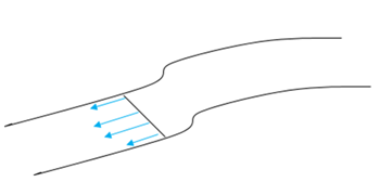
Fig no 9 Velocity Distribution in Broadcasting

Although frequently used in river engineering activities, the legitimacy of the prandtl curve and equation (1) is not considered normal, in fact many proposed species intended to describe this distribution "with greater accuracy" than (1) .10 This would have been apparent if the Grandtl curve had not been recognized as its only potential. Within the foundation of the body. This recognition is expressed in the following way.

Leopold's view of the “Stable” Streams: The goal of steady flow

L. Leopold (Albuquerque 1915, Berkeley 2006) likewise was a famous American scientist who contributed to the effective application of I.Prigogine's ideas on river hydraulic hydration. It is because of the observation that, in "natural flow" in the stable state ", the normal velocity is the same at birth and in the delta", i.e., "the intensity of the medium velocity in the natural flow (Leopold's goal).

Thermodynamic Description of Leopold's Principle

Although Leopold did not support his Principle in addition to an exploratory observation on a large number of rivers in the USA, it is not hard to point out that this statement is based on the principles outlined by I.Prigogine (also used by Leopold). 11 Therefore, based on the principle of "Equiprobability" to flow "in a reliable state" near equity, it can be seen that if potential power is distributed throughout the system volume in a "tangible" way, then the transfer of magnitude from one point to another in this phase is equal. All points, so the velocities are equal. Medium speed fluctuations in "all flow" (long lengths) are then given as a result of thermodynamics of non-adjustable processes.

The application of Leopold's principle to dynamic energy in a dynamic sense

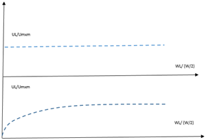
At longer distances Leopold's law is valid, especially at shorter distances. Therefore, not only in the long-term sense is the validity of the flow rate in "Equiprobability" valid but also in a flexible manner. Therefore, the distribution of the longitudinal velocity is the same, meaning that it is a straight line (the velocities in this axis), as above Figure 4. If you look at the viscosity acting on the wall area, this distribution deviates as in Figure 4. Then, the Prandtl curve it is actually the result of the Constancy Principle of velocity in the thermodynamic system considered, and in this sense is a general definition, which can be met by other models of different velocity distribution.

Fig no 10 Leopold principle and prandtl deflection

Key takeaways

Distribution of lateral velocities lateral veins

This concept is illustrated in Figure

Several models represent this distribution

8.12 Resistance to Flow of Fluid in Smooth And Rough Pipes

When a fluid flows through a pipe, frictional resistance is offered to the motion of the fluid and the loss of head due to friction is expressed by Darcy- Weishach equation,

But the loss of head can be predicted correctly only if the friction coefficient can be evaluated accurately.

It can be shown by dimensional analysis that the friction coefficient depends upon the Reynolds number

. and the ratio k/D

Thus,

Where, D = Diameter of the pipe

= Density of the fluid.

= Dynamic viscosity of the fluid.

K= average height of pipe wall roughness protrusions.

The term K / D is commonly known as relative roughness.

The equation 1 general equation which is applicable to laminar as well as turbulent flow in pipes.

Variation of friction coefficient f for smooth pipe-

The coefficient of friction f for turbulent flow in both pipes is a function of Reynolds number only and is independent of relative roughness K / D.

The value of f for smooth pipes for Re varying from 4000 to 105 is given by the following empirical relation.

The values of f for Re

105 to Re = 4 × 107obtained by using following equation.

Nikuradse’s experimental result for turbulent flow in smooth pipe For Re = 5×10⁴ to Re as high as 4 × 107 for f is

f =

Variation of friction coefficient f for rough pipes

For turbulent flow in rough pipes, the friction coefficient f depends only on relative roughness (K/D) and is independent of Reynolds Number (Re). An expression for f is as follows:

The experimental results obtained by Nikuradse follows the trend of following equation.

Examples:

Q.1 A pipeline of 0.3 diameter carries liquid at the rate of 0.540 m/s. If the sp. gravity of the liquid is 0.80 and its kinematic viscosity is 0.023 x 10 m/s, determine the maximum permissible height of the protrusions up to which the pipe acts as smooth pipe and the height of the protrusions beyond which the pipe would become rough.

Soln.:

Given: d=0.3 m, Q=0.543 m/s

R= d/2 = 0.3 /2 = 0.15m

Average velocity of flow

Reynold's number

Turbulent flow for smooth pipe for Re

Relation for friction factor

Solving above equation, we get f = 0.0113

Permissible height of the protrusions

Q.2 In a pipe of diameter 300 mm the centre line velocity and the velocity at a point 100 mm from the centre, as measured by pitot tube are 2.4 m/sec and 2 m/sec respectively, assuming the flow in the pipe to the turbulent find:

(1) Discharge through pipe

(2) Coefficient of friction

(3) Height of roughness projection.

Soln.:

Given:

Diameter d 300 mm=0.3 m,

Radius R 150 mm = 0.15 m

Velocity at centre u max = 2.4 m/sec.

Velocity at r=100=0.1 m;

u= 2 m/sec y=R-r=0.05 m

Step 1: Now for turbulent flow,

Step 2: The relation between velocity at any point and average velocity, at y R, u= u max

Step 3: Discharge,

Q = Area x Average velocity

Step 4: Coefficient of friction,

Step 5: Height of roughness projection, by using Karman-Prandtl resistance equation for rough pipe is, Use f4f (Friction factor f4 x Coefficient of friction)

K=6.324 mm

Key takeaways

Variation of friction coefficient for smooth pipes

f =

Variation of friction coefficient for rough pipes

8.13 Moody's Diagram

We know, Friction factor for laminar region is governed by the formula;

And for the turbulent region, it is governed by the Colebrook’s empirical relation;

Based on the above two equations, following figure was prepared.

It shows the functional dependence of friction factor (f) on Reynold’s no. (Re) and relative roughness (

and is called as moody’s chart in honor of L.F. Moody who along with C.F. Colebrook, correlated the original data of Nikuradse in terms of relative roughness of commercially available pipes and prepared the chart.

Roughness values of some commercial pipes are shown on Moody’s chart.

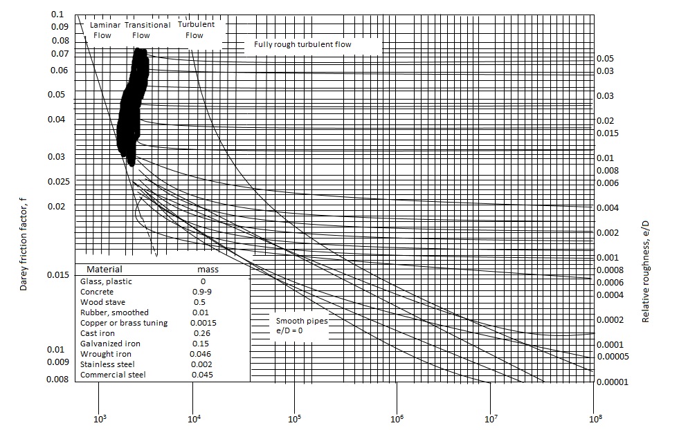
Fig no Moody chart

But it should be kept in mind that these values are for new pipes, and the relative roughness of the pipes may increase with use as a result of corrosion and scale build up.

Following observations can be made from Moody’s chart:

For laminar flow, the fraction factor decreases with increase in Reynold’s Number, and it is independent of relative roughness.

At very large Reynold’s Number, the friction factor curves corresponding to specified relative roughness are nearly horizontal, and thus the friction factors are independent of Reynolds’s Number.

For flow with moderate values of Re, the friction factor is indeed dependent on both the Reynold’s number as well as relative roughness and the value can be read from the chart.

Note that even for smooth pipe (ε = 0); the friction factor is zero. That is, there is head loss in any pipe, no matter how smooth the surface is made. This is due to no slip condition at the pipe wall.

This transition region from laminar to turbulent region (2300 < Re < 4000) is indicated on the chart. The flow in this region may be laminar or turbulent depending on the flow disturbances.

It is probably one of the most widely accepted and used charts in engineering. Although it was developed for circular pipes, it can also be used foe non-circular pipes by replacing the diameter with hydraulic diameter.

Also, the Moody’s chart involves various inherent inaccuracies and thus results obtained should not be treated as exact.

It is usually considered to be accurate to ±15% over the entire range in the figure.

Examples:

Q.1 Determine the head loss in kPa for a pipe line 700 m long carrying petrol at the flow rate of 200 Lps. (p = 730 kg/m³, μ = 2.92 x 10 N-s/m²). The diameter of the pipe is 30 cm and the equivalent roughness magnitude is 0.3 mm. Use Moody's diagram.

Soln.:

Given: L = 700 m long,

Q = 200 Lps= 0.2 m³/sec,

p = 730 kg/m³, μ = 2.92 x 10 N-s/m².

d = 30 cm = 0.3 m, e = 0.3 mm = 0.3 x 10³ m

Step 1: Velocity,

Step 2: Relative roughness,

Step 3: Reynolds’s number,

Step 4: Refer Moody's diagram and R., we get

Step 5: Head loss by Darcy's equation,

Step 6: Head loss in kPa (pressure),

= 132.98 x 10³ mPa

p = 132.98 kPa

:. The head loss in kPa is 132.98 kPa.

Q.2 Determine the head lost in a diameter 300 m, 300 m long cast iron pipe when (1) Water at 15°C flow at a velocity 15 nvs and (ii) Fuel oil at 15°C flow at the same velocity. Assume size of surface imperfection 0.244 mm. Refer Moody's diagram. Take the following properties.

Fluid	Density (kg/m^3 )	Viscosity (m^2/s)
Water	999.1	1.141x10^-6
Fuel oil	858	4.41x10^-6

Soln.:

Given:

L = 300 m, d = 300 mm = 0.3 m,

c = 0.244, V = 15 m/sec.

Case I: When water is flow with velocity = 15 m/sec.

e = 0.244

Step 1: Relative roughness

Step 2: Reynolds number

Step 3: Use moody's table for R. and values,

f = 0.0186

Step 4: Head loss by Darcy's equation,

Case II: When oil flows with same velocity 1.5 m/sec,

:. By using Moody's curve for Re and e/d values,

f = 0.0215

Head loss

Key takeaways

It shows the functional dependence of friction factor (f) on Reynold’s no. (Re) and relative roughness ( and is called as moody’s chart in honor of L.F. Moody who along with C.F. Colebrook, correlated the original data of Nikuradse in terms of relative roughness of commercially available pipes and prepared the chart.

Also, the Moody’s chart involves various inherent inaccuracies and thus results obtained should not be treated as exact.

References:

Fluid mechanics and machinery R Berndtsson and P.N. Chadramouli

Hydraulic and fluid mechanics, PM Modi and SM Seth

Theory and applications of fluid mechanics, K Subramanya, Tata McGraw Hill

Fluid mechanics with engineering applications, RL Daughterty, JB Franzini

Sign Up

Index

Notes

Highlighted

Underlined

Browse by Topics

Notes

Highlighted

Underlined