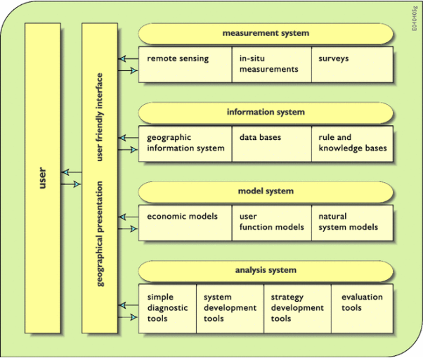
Unit 6

Computational Fluid Dynamics

6.1           Basic equation of fluid dynamics-

• The main task in fluid dynamics is to find the velocity field describing the flow in a given domain. To do this, one uses the basic equations of fluid flow, which we derive in this section.
• These encode the familiar laws of mechanics:

1. Conservation of mass
2. Conservation of momentum
3. Conservation of energy

      Conservation of mass:

• The continuity equation:

Consider a volume V bounded by a surface S that is fixed in space. This mass in side it is given by, so the

Rate of decrease of mass in V = - = -dV

If mass is conserved, Eqn. 1 must equal the total rate of mass flux out of V. How do we calculate this? The rate of outward mass flux across any small element dS of S is ρvdS where the magnitude of dS is equal to the element’s area and we take dS along the outward normal. Integrating over the whole surface we have

Rate of mass flux out of V = =

Where, we used Green’s formula to convert to a volume integral. The integrand ∇(ρv)on the RHS is expressed in Cartesian coordinates x= (x, y, z), v= (u, v, w) as

= + +

The continuity equation is,

+ = 0

      Conservation of momentum:

• The Cauchy equations:

Consider a volume V bounded by a material surface S that moves with the flow, always containing the same material elements. Its momentum is, so:

Rate of change of momentum = =

(The mass ρdV of each material element is constant.) This must equal the net force on the element. Actually there are two different types of forces that act in any fluid:

Long range external body forces that penetrate matter and act equally on all the material in any element dV. The only one considered here is gravity.

For any element, the net effect of these due to interactions with other elements acts in a thin surface layer. In 3D, each of the 3 sets of surface planes bounding an element experiences a 3-component force, giving 9 components in all. These form the stress tensor [Π], defined so the force exerted per unit area across a surface element S ≡ ndS (by the fluid on the side to which n points on the fluid on the other side) is f= [Π]·ˆn.

Total force (body + surface) =

=

By Newton’s second law, so we get finally

The Cauchy Equation:

= +

• Boundary conditions:

In any flow domain, the flow equations must be solved subject to a set of conditions that act at the domain boundary. For a rigid bounding wall moving at velocity U and having unit normal n, we assume for the local fluid velocity v that1. The wall is impermeable: v·ˆn=U·ˆn.2. The fluid doesn’t slip relative to the wall: v׈n=U׈n. Condition 2 is not obvious: why shouldn’t slip occur? The underlying notion is that the fluid interacts with the wall in the same way as with other fluid: there cannot live any discontinuity in velocity, or an infinite viscous stress would arise. But the ultimate justification comes from experimental verification.

6.2           Grid generation

Grid:-

A basic concept of CFD is to divide the fluid geometry into elements or cells, and then solve an equation for each cell. In the following text, the word cell will be used instead of element, to avoid confusion with the finite element method.

• Classifications of Grid:
• Grids can be classified according to several characteristics:

1. Shape
2. Orthogonal structure
3. Structure
4. Blocks
5. Position of variable
6. Grid movements

The shape of the cells is usually triangular or quadrilateral.

Elliptic grid generation:

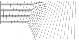
• Elliptic grid generation is a method to distribute internal points smoothly in a structured quadrilateral grid. This is done by solving a Laplace or Poisson equation for the location of the grid line intersections. The location of the grid lines are denoted ξ. P is a source term used for attracting grid lines to a side or a point.
• This grid is made by use of transfinite interpolation. This means that straight lines are made between the points on the wall.

Elliptic procedures are used to obtain the grid shown above, with no attractions.

• Elliptic procedures are used to obtain the grid shown above, with no attractions. Looking at the lower point of the step, the cells are smaller closer to the wall. This is due to attraction functions.

Practical advice for generating structured non-orthogonal grids:

• Making a good grid is a considerable part of the work for CFD calculations for complex geometries. Experience seems to be very important for this task, so the first advice is to practice making grids. Before starting to make the grid, some information is necessary:

1. How many grid cells are available for the grid? This can be calculated from the capacity of the computer and the expected computational time.

2. Drawings of the geometry are important, where boundaries and the inflow/outflow regions are shown together with possible islands or other out blocked regions. An out blocked region is a part of the grid where water is not allowed to flow. It can be used for making islands or obstacles in the flow.

• An example is given below with flow around a square obstacle:

Note that not all computer programs have the option of blocking out parts of the grid. If the geometry is complex, one should make a paper sketch of the grid before starting to use the computer. The paper sketch should be reasonably large in order for the details to be visible.

• The boundary of the grid should be marked with one colour and inflow/outflow regions with another colour. One should start with deciding the general structure of the grid: where the four sides of the grid should be located.
• If out blocking is needed and possible, this should be decided together with the location of the out blocking in the grid.

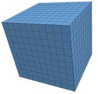
• Then one should start drawing the grid, using a pencil and an eraser, as modifications are always needed. One should preferably start making a very coarse grid, maybe with only 6-12 cells, and making the grid finer afterwards. When drawing the grid, the following points should be kept in mind.

1. The grid lines should follow the stream lines as much as possible

2. The grid line intersections should be as orthogonal as possible

3. The grid aspect ratio should not be too great

4. The grid expansion ratio should not be too great

5. There should be higher grid densities in areas with high velocity/concentration gradients. In a not too complex part of a river, the gradients in cross-stream wise direction are larger than in the stream wise direction. The grid cells can then be longer in the stream wise direction than in the cross stream wise direction. An example is given in the figure below, where the aspect ratios for the cells are above unity.

• After having made the paper sketch of the grid, the tools of the CFD computer pro-gram can be used to make the final grid.
• Note that the same points as given above apply when using the grid tools of the CFD program.

Computational fluid dynamics: Basic equation of fluid dynamics:

Computational fluid dynamics or CFD is the analysis of systems involving fluid flow, heat transfer and associated phenomena such as chemical reactions by means of computer-based simulation. The technique is very powerful and spans a wide range of industrial and non-industrial application areas. Some examples are

• Aerodynamics of aircraft and vehicles: lift and drag
• Hydrodynamics of ships
• Power plant: combustion in internal combustion engines and gas turbines
• Turbo machinery: flows inside rotating passages, diffusers etc.
• Electrical and electronic engineering: cooling of equipment including       micro circuits
• Chemical process engineering: mixing and separation, polymer moulding• external and internal environment of buildings: wind loading and heating/ventilation
• Marine engineering: loads on off-shore structures
• Environmental engineering: distribution of pollutants and effluents
• Hydrology and oceanography: flows in rivers, estuaries, oceans
• Meteorology: weather prediction
• Biomedical engineering: blood flows through arteries and veins

From the 1960s onwards the aerospace industry has integrated CFD techniques into the design, R&D and manufacture of aircraft and jet engines. More recently the methods have been applied to the design of internal combustion engines, combustion chambers of gas turbines and furnaces. Furthermore, motor vehicle manufacturers now routinely predict drag forces, under-bonnet air flows and the in-car environment with CFD. Increasingly CFD is becoming a vital component in the design of industrial products and processes. The ultimate aim of developments in the CFD field is to provide a capability comparable with other CAE (computer-aided engineering) tools such as stress analysis codes.

The main reason why CFD has lagged behind is the tremendous complexity of the underlying behaviour, which precludes a description of fluid flows that is at the same time economical and sufficiently complete. The availability of affordable high-performance computing hard-ware and the introduction of user-friendly interfaces have led to a recent upsurge of interest, and CFD has entered into the wider industrial community since the 1990s.

6.3           Introduction to viscid incompressible flow:

• In fluid dynamics, a flow is considered incompressible if the divergence of the flow velocity is zero. However, related formulations can sometimes be used, depending on the flow system being modelled.
• In viscid flow is the flow of an in viscid fluid, in which the viscosity of the fluid is equal to zero. Though there are limited examples of in viscid fluids, known as super fluids, in viscid flow have many applications in fluid dynamics. Such a flow has no viscous resistance to its motion.
• Example of incompressible fluid flow: The stream of water flowing at high speed from a garden hose pipe. Which tends to spread like a fountain when held vertically up, but tends to narrow down when held vertically down?  The reason being volume flow rate of fluid remains constant.
• The stream of water flowing at high speed from a garden hose pipe. Which tends to spread like a fountain when held vertically up, but tends to narrow down when held vertically down? The reason of being volume flow rate of fluid remains constant.

      Kinematic Definitions:

The position vector of a fluid particle at time t is denoted as

r= (x, y, z) = xi+ yj+ zk,

Where i, j, k are the usual Cartesian unit vectors. The velocity of a fluid particle is denoted as

u= (u, v, w) = ui + vj + wk.

Alternatively, we can write r = xiei, u = uiei

Where i= 1, 2, 3, is the unit vector along the Cartesian a xi s xi and the summation convention over repeated indices is used so that, for example xiei = 3∑i=1xiei.

There are two common approaches to describing the flow.

Lagrangian specification: all the relevant quantities (e.g. Position vector, velocity, acceleration etc.) for a chosen fluid particle are functions of time and the position of the particle at some initial time, for instance at t= 0.For example, if r0 is the position vector of a fluid particle at time t= 0, then the position vector of the same particle at time t will be r = r (r0 t).

6.4           Boundary layer flow as applicable to CFD:

• In recent years wind energy as a percentage of total energy consumed in Sweden has increased substantially. During the ten year span from 2006 to 2016 this percentage has gone from 1% to 15%. As wind farms have quickly occupied the most optimal locations for wind energy generation there is an increasing need to occupy less optimal areas. However, poorly sited wind farms may yield costly energy production due to high maintenance and/or inefficient energy production.
• In order to assess the quality of potential sites, on-site measurements are used but they can only provide local values which are of limited use when compared to how large wind patterns are. This raises a demand for accurate computer simulations which can predict well the structures and patterns in atmospheric wind flows. Simulation techniques for wind turbine responses are accurate and computation-ally inexpensive.
• Their accuracy is however completely dictated by an accurate description of the incoming wind pattern. In simple cases the wind patterns maybe replicated to a high degree of accuracy but as the terrain increases in complexity so do the wind patterns.
• With modern computational power the time-average of these complicated patterns can be predicted with fair accuracy using CFD models. Because of the turbulent (seemingly random) behaviour of the wind patterns these time-averaged results prove insufficient for use when predicting fatigue loads on a turbine blade or other components of a wind turbine.
• This is where transient model simulations may excel, at the added cost of computational power.
• This study will focus on generating a transient CFD model of atmospheric boundary layer flow to study the effects of complex terrain on the dynamic response of a wind turbine.

The main objectives and limitations of this study have been summarised in the following list:

• Utilise CFD models known to predict well the time-averaged behaviour of a neutral atmospheric boundary layer to assess the shape of flow structures.
• Using the time-averaged results as reference, establish a CFD model to predict the transient behaviour of the neutral atmospheric boundary layer.
• Study the dynamic response of a wind turbine using the transient generated wind fields combined with aero-elastic solver.
• Quantify the main differences found between the flow over flat and complex terrains in terms of the flow and the response of the wind turbine.
• The quality of the transient flows simulated is only evaluated against mean flows generated with CFD as opposed to actual measurements. The CFD study is limited to the use of Star-CCM+ and the models it provides.
• The CFD study is limited by the amount of computational resources available.

6.5           Concept of hydro-informatics:

Scope of internet and web based modelling in water resource engineering:

• Hydro-informatics, as an interdisciplinary domain that blurs boundaries between water science, data science and computer science, is constantly evolving and reinventing itself. At the heart of this evolution, lies a continuous process of critical (self) appraisal of the discipline’s past, present and potential for further evolution that creates a positive feedback loop between legacy, reality and aspirations.
• The power of this process is attested by the successful story of hydro-informatics thus far, which has arguably been able to mobilize wide ranging research and development and get the water sector more in tune with the digital revolution of the past 30 years.
• In this context, this paper attempts to trace the evolution of the discipline, from its computational hydraulics origins to its present focus on complete socio-technical system, by providing at the same time, a functional frame work to improve the understanding and highlight the links between different strands of the state-of-art hydro-informatics research and innovation. Building on this state-of-art landscape, the paper then attempts to provide an overview of key developments that are coming up, on the discipline’s horizon, focusing on developments relevant to urban water management, while at the same time, highlighting important legal, ethical and technical challenges that need to be addressed to ensure that the brightest aspects of this potential future are realized. Despite obvious limitations imposed by a single paper’s ability to report on such a diverse and dynamic field, it is hoped that this work contributes to a better understanding of both the current state of hydro-informatics and to a shared vision on the most exciting prospects for the future evolution of the discipline and the water sector it serves.
• Water systems and services are highly complex as they are tasked to balance water resources with demands through complex interconnected infrastructure. As such, decision making about these systems and services (at strategic, tactical and operational scales) need to be taken within a continuously changing landscape where water quality and quantity are uncertain.
• These systems are also influenced by climatic changes and human practices water demand patterns are shifting as urbanization continues, influencing demands as standards of living rise. Lastly environmental legislation and customer expectations are also shifting and with them, the thresholds against which the water sector’s performance is measured also change. This dynamic decision landscape is further complicated by aging infrastructure and the advent of new (disruptive) technologies and concepts
• Hydro-informatics is a branch of informatics which concentrates on the application of information and communications technologies (ICTs) in addressing the increasingly serious problems of the equitable and efficient use of water for many different purposes. Growing out of the earlier discipline of computational hydraulics, the numerical simulation of water flows and related processes remains a mainstay of hydro-informatics, which encourages a focus not only on the technology but on its application in a social context.
• On the technical side, in addition to computational hydraulics, hydro-informatics has a strong interest in the use of techniques originating in the so-called artificial intelligence community, such as artificial neural networks or recently support vector machines and genetic programming. These might be used with large collections of observed data for the purpose of data mining for knowledge discovery, or with data generated from an existing, physically based model in order to generate a computationally efficient emulator of that model for some purpose.
• Hydro-informatics recognises the inherently social nature of the problems of water management and of decision making processes, and strives to understand the social processes by which technologies are brought into use. Since the problems of water management are most severe in the majority world, while the resources to obtain and develop technological solutions are concentrated in the hands of the minority, the need to examine these social processes are particularly acute.
• Hydro-informatics draws on and integrates hydraulics, hydrology, environmental engineering and many other disciplines. It sees application at all points in the water cycle from atmosphere to ocean and in artificial interventions in that cycle such as urban drainage and water supply systems. It provides support for decision making at all levels from governance and policy through management to operations.

      Web based modelling in water resource engineering:

• Modelling provides a way, perhaps the principal way, of predicting the behaviour or performance of proposed system infrastructure designs or management policies. The past 50 years have witnessed major advances in our abilities to model the engineering, economic, ecologic, hydrologic, and sometimes even the institutional or political aspects of large complex multipurpose water resource systems.
• Applications of models to real systems have improved our understanding of such systems, and hence have often contributed to improved system design, management, and operation. They have also taught us how limited our modelling skills remain.

• Water resource systems are typically far more complex than what analysts can model and simulate. The reason is not primarily due to computational limitations but rather it is because we do not understand sufficiently the multiple interdependent physical, bio chemicals, ecological, social, legal, and political (human) processes that govern the behaviour of such water resource systems. People and their institutions impact the performance of such systems, and the performance of these systems impacts people.
• System performance is affected by uncertainties in things we can measure and processes we can predict. They are also affected by the unpredictable actions of individuals and institutions as they manage and use water in response to a multitude of impacts they experience in their physical and social environment. Some of these impacts are water related. Others have nothing directly to do with water.

      Modelling Water Resource Systems:

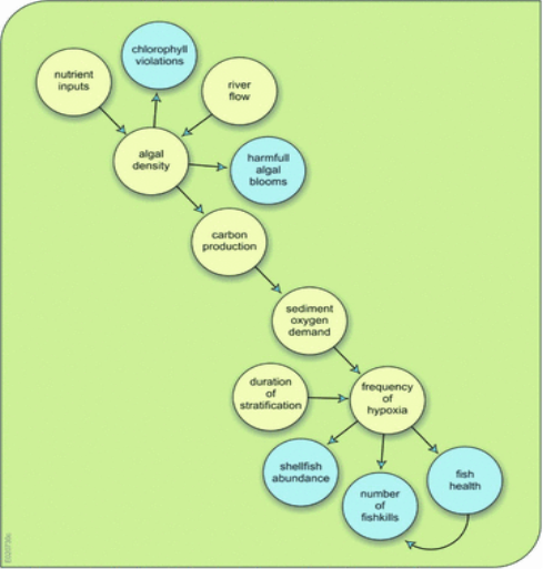
• Consider for example the sequence or chain of models illustrated in Fig. required for the prediction of fish and shellfish survival as a function of nutrient loadings into an estuary. The condition of the fish and shellfish are important to the economy of the region and the income of many stakeholders. One way to maintain healthy stocks is to maintain sufficient levels of oxygen in the estuary.
• The way to do this is to control algae blooms. This in turn requires limiting the nutrient loadings to the estuary that can cause algae blooms and subsequent dissolved oxygen deficits. The modelling challenge is to link nutrient loading to fish and shellfish survival. In other words, can some quantitative relationship be defined relating the amount of nutrient loading to the amount of fish and shellfish survival?

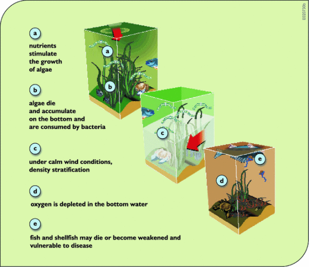
• The negative effects of excessive nutrients (e.g., nitrogen) in an estuary are shown in Fig. Nutrients stimulate the growth of algae. Algae die and accumulate on the bottom where bacteria consume them. Under calm wind conditions density stratification occurs. Oxygen is depleted in the bottom water. As a consequence, fish and shellfish may die or become weakened and more vulnerable to disease.
• A sequence of models, each providing input data to the next model, can be defined to predict shellfish and fish abundance in the estuary based on upstream nutrient loadings. These models, for each link shown in Fig. Can be a mix of judgmental, mechanistic, and/or statistical ones. Statistical models could range from simple regressions to complex artificial neural networks. Any type of model selected will have its advantages and its limitations. Its appropriateness may largely depend on the amount and precision of the data available for model calibration and verification.
• The results of any modelling exercise should be expressed in terms meaningful and of interest to those that will be making decisions taking into account those results. In this example ‘shell-fish abundance’ and ‘number of fish-kills’ are meaningful indicators to stakeholders and can be related to designated water body use.

      Characteristics of Problems to be modelled:

• Problems motivating modelling and analyses exhibit a number of common characteristics. These are reviewed here because they provide insight into whether a modelling study of a particular problem may be worthwhile. If the planners’ objectives are very unclear, if few alternative courses of action exist, or if there is little scientific understanding of the issues involved, then mathematical modelling and other more sophisticated methodologies are likely to be of little use.

Successful applications of modelling are often characterized by:

•         A systems focus or orientation. In such situations attention needs to be devoted to the interdependencies and interactions of elements or components within the system as a whole, as well as to the elements or components themselves.

•         The use of interdisciplinary teams. In many complex and non-traditional problems, it is not at all clear from the start what mix of disciplinary viewpoints will turn out to be most appropriate or acceptable. It is essential that participants in such work—coming from different established disciplines—become familiar with the techniques, vocabulary, and concepts of the other disciplines involved. Participation in interdisciplinary modelling often requires a willingness to make mistakes at the fringes of one’s technical competence and to accept less than the latest advances in one’s own discipline.

•         The use of formal mathematics. Most analysts prefer to use mathematical models to assist in system description and the identification and evaluation of efficient trade-offs among conflicting objectives, and to provide an unambiguous record of the assumptions and data used in the analysis.

•         The planning and management objectives are reasonably well defined, and organizations and individuals can be identified who can benefit from obtaining and understanding the model results.

•         There are many alternative decisions that may satisfy the stated objectives, and the best decision is not obvious.

•         The water resources system and the objectives being analysed are describable by reasonably tractable mathematical representations.

•         The information needed, such as the hydrological, economic, environmental, and ecological impacts resulting from any decision, can be better estimated through the use of models.

•         The values of the model parameters are estimable from readily obtainable data.

      Challenges of Planners and Managers:

• Planners and managers of water resource systems are responsible for solving particular water-related problems or meeting special water resource needs. When they fail, they hear about it. The public lets them know. (Example: the lead contamination in the drinking water of Flint, Michigan USA, after a switch in the water source to reduce costs.) What makes their job particularly challenging is that stakeholders often have different needs and expectations. Furthermore, institutions where water resource planners and managers work (or hire consultants to work for them) are like most institutions these days. They must do what they have been asked to do with limited financial and human resources. Their clients include all of us who use water, or at least all of us who are impacted by the decisions they make.
• The overall objective of planners, managers, and operators and their institutions is to provide a service, such as reliable and inexpensive supplies of water, assurance of water quality, production of hydropower, protection from floods, provision of commercial navigation and recreational opportunities, preservation of wildlife and enhancement of ecosystems, or some combination of these or other purposes. Furthermore they are expected to do this at a cost no greater than what people are willing to pay. Meeting these goals, i.e., keeping everyone happy, is not always easy, or even possible.
• Simple technical measures or procedures are rarely available that will ensure a successful solution to any particular set of water resource management problems. Furthermore, everyone who has had any exposure to water resources planning and management knows one cannot design or operate a water resource system without making compromises. These compromises often involve competing purposes (such as hydropower and flood control) or competing objectives (such as who benefits and who pays, and how much and where and when). After analysts, using their models of course, identify possible ways of achieving various goals and objectives and provide estimates of associated Economical, environmental, ecological, and social impacts, it is the decision-makers who have the more difficult job. They must work with and influence everyone who will be affected by any decision.
• Moving an organization or institution into action to achieve specific goals involves a number of activities, including goal-setting, debating, coordinating, motivating, deciding, implementing, and monitoring. Many of these must be done simultaneously and continuously, especially as conditions (goals and objectives, water supplies, water demands, financial budgets) change over time. These activities create a number of challenges that are relevant to modellers or analysts. Some include:

1. Identifying creative ways of solving problems.

2. Finding out what each interest group wants to know in order to reach an understanding of the issues and a consensus on what to do.

3. Developing and using models and presenting their results so that everyone can reach a common or shared understanding and agreement that is consistent with their individual values.

4. Making decisions and implementing them given differences in opinions, social values, and objectives.

In addressing these needs or challenges, planners, and managers must consider the relevant

• Legal rules and regulations;
• History of previous decisions;
• Preferences of important actors and interest groups;
• Probable reactions of those affected by any decision;
• Relative importance of various issues being addressed; and finally;
• Sciences, engineering, and economics—the technical aspects of their work.
• This traditional modelling process is clearly not going to work for those who are not especially trained or experienced or even interested in these modelling activities. They need a model-building environment where they can easily create models that

• They understand,
• Are compatible with available data,
• Work and provide the level and amount of information needed,
• Are easily calibrated and verified when possible, and
• Give them the interactive control over data input, editing, model operation and output display that they can understand and need in order to make informed decisions.