Unit – 3
Linear Prediction of Speech
In almost all modern speech coding algorithms, linear prediction (LP) is a key component. A speech sample can be approximated as a linear combination of previous samples, according to the basic concept. The weights used to calculate the linear combination within a signal frame are determined by reducing the mean-squared prediction error; the resulting weights, or linear prediction coefficients (LPCs*), are used to represent the frame.
The autoregressive model is at the heart of the LP system. Indeed, linear prediction analysis is an estimation technique for determining AR parameters from signal samples. As a result, LP is an identification technique in which device parameters are discovered by observation. The basic premise is that speech can be modeled as an AR signal, which has proven to be accurate in practice.
Another way to look at LP is as a spectrum estimation technique. As previously mentioned, LP analysis allows for the computation of the AR parameters, which determine the signal's PSD. It is possible to produce another signal with spectral contents that are similar to the original by computing the LPCs of a signal frame.
LP may also be thought of as a redundancy-removal process, in which redundant information in an incident is removed. After all, if such data can be expected, there is no need for transmission. The amount of bits needed to hold the information is reduced when redundancy in a signal is displaced, achieving the compression goal.
The fundamental problem of LP analysis is defined, followed by its application to nonstationary signals. There are examples of processing on real-world speech recordings. LP isn't just for speech processing; it's used in a wide range of applications.
Key takeaway:
The LPCs must be determined for each signal frame due to the complex existence of speech signals. One collection of LPCs is calculated and used to display the signal's properties in that specific interval within a frame, with the underlying assumption that the signal's statistics do not shift within the frame. Linear prediction analysis is the method for computing LPCs from signal data.
The linear prediction problem is rephrased as follows: The LPCs on the N data points ending at time m should be calculated as follows: s[m - N + 1], s[m - N + 2],... ;s[m]. The LPC vector looks like this:
a[m] = [a1[m] a2[m] …………. aM[m]]T
M denotes the prediction order. We need to solve the usual equation, which has been rewritten in a time-adaptive form.
R[m]a[m] = -r[m]
With,

And
r[m] = [R[1, m] R[2; m] R[M, m]]T
As a result, LP analysis is performed for any signal frame ending at time m in the case of non stationary signals. For each frame, the autocorrelation values R[l, m] are calculated, and the usual equation is solved to produce the collection of LPCs associated with that frame.
3.2.1 Prediction Gain
Prediction benefit is calculated using a similar concept as before, with the exception that the assumptions are now summations.

Where,

The LPCs ai[m] was discovered from samples falling within the interval [m - N + 1, m] for internal prediction and n < m N + 1 for external prediction. It's worth noting that the prediction benefit is a function of the time variable m. In practice, the segmental prediction benefit, which is described with, is frequently used to assess a prediction scheme's overall performance.
SPG = A{PG[m]}
In the decibel domain, this is the time average of the prediction gain for each frame.
3.2.2 Examples
When using a speech signal, it's common to believe that the signal would satisfy the AR model. In this section, facts about LP analysis of speech are extracted from actual speech samples, and the accuracy of the AR assumption is assessed. The findings are used to tailor the LP scheme as it relates to speech coding.
Example:
The experiment uses speech samples from a male participant. The speech frames that were considered are shown in Figure 1. As can be seen, the frame ending at m = 400 is unvoiced, while the frame ending at m = 1000 is voiced, with a pitch interval of around 49 time-units in between.
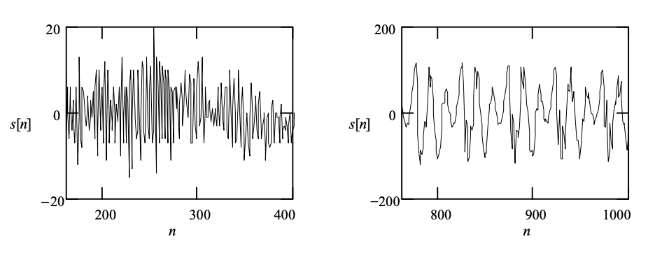
Fig 1: The speech frames used in the experiment. Left: Unvoiced (m = 400). Right: Voiced (m = 1000)
It's also worth noting that the unvoiced frame has a far lower amplitude than the voiced frame, which is often the case in practice. Each frame is 240 samples long, which is a common value in speech coding. Figure 2 shows the periodograms of the two frames.
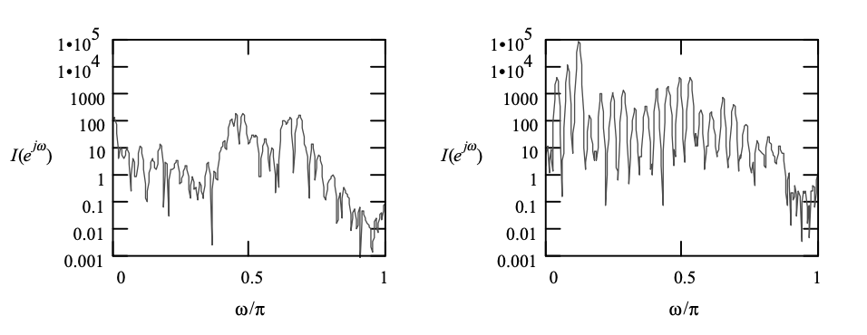
Fig 2: Periodograms of the signal frames in Figure 4.6. Left: Unvoiced. Right: Voiced.
The unvoiced frame's spectrum is relatively smooth, while the voiced frame's spectrum has a harmonic structure, suggesting a strong fundamental component in the signal. Harmonics are obviously linked to periodicity in the time domain.
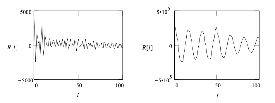
Fig 3: Autocorrelation values for the signal frames in Figure 4.6. Left: Unvoiced. Right: Voiced.
The autocorrelation values shown in Figure 3, where the lag ranges from 0 to 100, can also be used to detect or quantify periodicity. The lag can be anywhere between 0 and 100. When the lag is greater than ten, the autocorrelation values for the noise-like unvoiced frame have a low magnitude, implying that correlation between distant samples is low. In the voiced picture, on the other hand, there is a high correlation between samples, which is particularly strong when the lag is equal to the pitch time, which in this case is about 49.
The value of the autocorrelation decreases with increasing lag in both cases, as predicted, since the correlation between samples weakens. These findings show that autocorrelation can be used to identify a frame as unvoiced or voiced, and pitch time can be calculated by locating the autocorrelation's peaks.
The chosen frames are subjected to LP analysis, with the resulting LPCs being used to predict the samples within the frame (internal prediction). The prediction benefit results are plotted in Figure 4 for prediction orders ranging from 2 to 100.
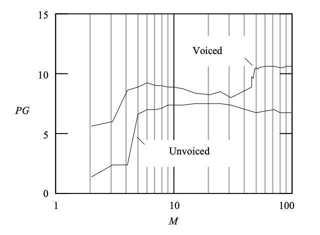
Fig 4: Plot of prediction gain (PG) as a function of the prediction order (M) for the signal frames in fig 1
Key takeaway:
With the solution given, the usual equation can be solved by finding the matrix inverse for Rs. In general, inverting a matrix is a computationally intensive operation. Fortunately, there are powerful algorithms for solving the equation that take advantage of the correlation matrix's unique structure. Consider the form's augmented normal equation.

The aim is to find a solution for the LPCs ai, i = 1,....., M given the autocorrelation values R[l], l = 0, 1,..., M. J represents the minimum mean-squared prediction error or variance of the input white noise for the AR process synthesizer. The autocorrelation values are normally calculated from signal samples in practice, and J is usually unknown; however, the Levinson–Durbin solution is formulated to solve for this quantity as well.
The Levinson–Durbin method extracts the Mth-order predictor's solution from the (M - 1)th-order predictor's. It's an iterative–recursive method in which the zero-order predictor's solution is first found, then used to find the first-order predictor's solution; this process is replicated one step at a time until the desired order is achieved. The algorithm is based on the correlation matrix's two main properties:
● All lower order correlation matrices are subblocks of a correlation matrix of a given size.
● If
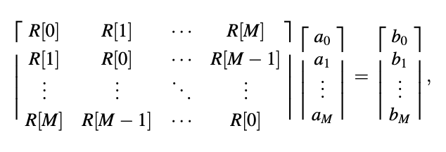
Then

That is, the correlation matrix is invariant when its columns and rows are swapped. The fact that the correlation matrix is Toeplitz has direct implications for the properties described. If all of the elements on the main diagonal of a square matrix are equal, and all of the elements on every other diagonal parallel to the main diagonal are also equal, we call it Toeplitz.
A Summary
The following is a description of the Levinson–Durbin algorithm. The autocorrelation coefficients R[l] are the algorithm's inputs, while the LPCs and RCs are the algorithm's outputs.
● Initialization: l = 0, set
J0 = R[0]:
● Recursion: for l = 1, 2, ... , M
Step 1. Compute the lth RC

Step 2. Calculate LPCs for the lth-order predictor:

Stop if l = M.
Step 3. Compute the minimum mean-squared prediction error associated with the lth-order solution
Jl = Jl-1 (1 - kl2)
Set l ← l + 1; return to Step 1.
The final LPCs are
ai = ai(M) i = 1, 2, ….., M
It's worth noting that while solving the LPCs, the set of RCs (ki, I 14 1, 2,..., M) is also discovered.
The Levinson–Durbin algorithm's computational efficiency is one of its advantages.
As opposed to traditional matrix inversion techniques, it results in a significant reduction in the number of operations and storage locations. Another advantage of its use is the collection of RCs that can be used to verify the resultant prediction-error filter's minimum phase property.
Key takeaway:
In order to accurately model the voiced signal under consideration, the prediction order must be high enough to include at least one pitch duration, according to real-world speech evidence. For example, a linear predictor with an order of ten cannot accurately model the periodicity of a voiced signal with a pitch period of 50. When looking at the prediction error, it's clear that there's a problem: the remaining periodic portion indicates a lack of fit.
The periodicity in the prediction error has largely vanished as a result of increasing the prediction order to include one pitch period, resulting in an increase in prediction gain. Since more bits are required to reflect the LPCs, and extra computation is required during analysis, a high prediction order results in an excessive bit rate and implementational expense. As a result, it is preferable to devise a scheme that is both straightforward and capable of accurately modeling the signal.
The first 8 to 10 coefficients, plus the coefficient at the pitch time, which in this case is 49, account for the majority of the increase in prediction gain. LPCs with orders between 11 and 48, as well as orders greater than 49, make no difference in terms of improving prediction gain. The flat segments from 10 to 49, and beyond 50, demonstrate this.
As a result, the coefficients that do not contribute to increasing the prediction gain can theoretically be removed, resulting in a more compact and efficient scheme. This is exactly the concept behind long-term linear prediction, in which a short-term predictor is linked to a long-term predictor in a cascade, as seen in Figure.

Fig 5: Short-term prediction-error filter connected in cascade to a long-term prediction-error filter.
The short-term predictor is essentially the same as the one we've been looking at so far, with a prediction order M in the range of 8 to 12. This indicator either removes the association between nearby samples or is temporally short-term. The long-term predictor, on the other hand, looks for association between samples that are separated by one pitch duration.
The machine feature of the long-term prediction-error filter with input es[n] and output e[n] is
H(z) = 1 + bz-T
The filter must be defined with two parameters: pitch duration T and longterm gain b. (also known as long-term LPC or pitch gain). Long-term LP analysis is the method used to evaluate b and T. The predictors' positions in Figure can literally be swapped.
The following pseudocode summarizes the step-by-step method of long-term LP analysis:
1. Jmin ← ∞
2. for T ← Tmin to Tmax
3. (Use (4.84) to compute b)
4. (Use (4.83) or (4.85) to compute J)
5. if J < Jmin
6. Jmin ← J
7. bopt ← b
8. Topt ← T
9. return bopt, Topt
In Line 2, the parameters Tmin and Tmax describe the search range for determining the pitch period. The reader should be aware that the pseudocode has not been optimized for speed. In reality, by examining the procedure's redundancy, the cost of computation can be significantly reduced.
Key takeaway:
The block diagrams of the AR process analyzer and synthesizer filters are shown in Figure 6, where a predictor with the difference equation is used. It's simple to confirm that these block diagrams produce the same equations for the AR model. Since a computationally efficient technique exists, parameters of the predictor are often found from the signal itself in realistic coding applications. This allows for real-time adaptation.

Fig 6: Block diagram of the AR analyzer filter (left) and synthesizer filter (right)
Figure 7 displays the analyzer and synthesizer filters' predictor-based block diagrams.

Fig 7: Block diagram of the MA analyzer filter (left) and synthesizer filter (right)
However, in this case, the predictor's difference equation is given by
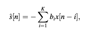
with K the order of the model and bi the MA parameters. Unlike the AR model, which can find the optimal parameters by solving a set of linear equations based on the statistics of the observed signal, the MA parameters can only be determined by solving a set of nonlinear equations, which is computationally intensive in practice.
As a result, other methods for determining model parameters are commonly used, such as spectral factorization and adaptive filtering techniques like the least-mean-square (LMS) algorithm, as well as other iterative methods.
LP is historically associated with AR modeling, despite the fact that it is a form of "linear prediction" scheme in which the prediction is based on a linear combination of samples. In the literature, prediction that is based on the MA model is referred to as ‘‘MA prediction."
Key takeaway:
References:
2. 2. “Speech Coding Algorithms: Foundation and Evolution of Standardized Coders”, W.C. Chu, Wiley Inter science, 2003.