Module 2 | unit 2 continuous probability distributions

Module -2

Continuous Probability Distributions

2.1 Continuous Random Variables:

A continuous random variable is a random variable where the data can take infinitely many values. For example, a random variable measuring the time taken for something to be done is continuous since there are an infinite number of possible times that can be taken.

Continuous random variable is called by a probability density function p (x), with given properties: p (x) ≥ 0 and the area between the x-axis & the curve is 1: ... Standard deviation of a variable Random is defined by σ x = √Variance (x).

A continuous random variable is known by a probability density function p(x), with these things: p(x) ≥ 0 and the area on the x-axis and the curve is 1:

∫-∞∞ p(x) dx = 1.

2. The expected value E(x) of a discrete variable is known as:

E(x) = Σi=1n xi pi

3. The expected value E(x) of a continuous variable is called as:

E(x) = ∫-∞∞ x p(x) dx

4. The Variance(x) of a random variable is known as Variance(x) = E[(x - E(x)2].

5. 2 random variable x and y are independent if E[xy] = E(x)E(y).

6. Standard deviation of a random variable is known as σx = √Variance(x).

7. Given value of standard error is used in its place of standard deviation when denoting to the sample mean.

σmean = σx / √n

8. If x is a normal random variable with limits μ and σ2 (spread = σ), mark in symbols: x ˜ N(μ, σ2).

9. The sample variance of x1, x2, ..., xn is given by-

sx2 =

(x1 - x)2 + ... + (xn - x)2

n - 1

10. If x1, x2, ... , xn are explanations since a random sample, the sample standard deviation s is known the square root of variance:

sx =

√

(x1 - x)2 + ... + (xn - x)2

n - 1

11. Sample Co-variance of x1, x2, ..., xn is known-

sxy =

(x1 - x)(y1 - y) + ... + (xn - x)(yn - y)

n - 1

12. A random vector is a column vector of random variable.

v = (x1 ... xn)T

13. Expected value of Random vector E(v) is known by vector of expected value of component.
If v = (x1 ... xn)T

E(v) = [E(x1) ... E(xn)]T

14. Co-variance of matrix Co-variance (v) of a random vector is the matrix of variances and Co-variance of component.
If v = (x1 ... xn)T, the ijth component of the Co-variance (v) is sij

Properties

Starting from properties 1 to 7, c is a constant; x and y are random variables.

E(x + y) = E(x) + E(y).
E(cx) = c E(y).
Variance (x) = E(x2) - E(x)2
If x and y are indiviadual, then Variance(x + y) = Variance (x) + Variance (y).
Variance (x + c) = Variance (x)
Variance(cx) = c2 Variance (x)
Co-variance (x + c, y) = Co-variance (x, y)
Co-variance (cx, y) = c Co-variance (x, y)
Co-variance (x, y + c) = Co-variance (x, y)
Co-variance (x, cy) = c Co-variance (x, y)
If x1, x2, ..., xn are discrete and N(μ, σ2), then E(x) = μ. We say that x is neutral for μ.
If x1, x2, ... , xn are independent and N(μ, σ2), then E(s) = σ2. We can told S is neutral for σ2.

From given properties 8 to 12, w and v is random vector; b is a continuous vector; A is a continuous matrix.

8. E(v + w) = E(v) + E(w)

9. E(b) = b

10. E(Av) = A E(v)

11. Co-variance (v + b) = Co-variance (v)

12. Co-variance (Av) = A Co-variance(v) AT

Probability Mass Function (PMF):

Let X be a D.R.V. Such that P(X=x) = P1 Then P1 is said to be probability mass function (p.m.f.) if it satisfy following condition:

(i)

(ii)

Probability Distribution:

A probability distribution is a arithmetical function which defines completely possible values & possibilities that a random variable can take in a given range. This range will be bounded between the minimum and maximum possible values. But exactly where the possible value is possible to be plotted on the probability distribution depends on a number of influences. These factors include the distribution's mean, SD, skewness, and kurtosis.

Probability Density:

Probability density function (PDF) is a arithmetical appearance which gives a probability distribution for a discrete random variable as opposite to a continuous random variable. The difference among a discrete random variable is that we check an exact value of the variable. Like, the value for the variable, a stock worth, only goes two decimal points outside the decimal (Example 32.22), while a continuous variable have an countless number of values (Example 32.22564879…).

When the PDF is graphically characterized, the area under the curve will show the interval in which the variable will decline. The total area in this interval of the graph equals the probability of a discrete random variable happening. More exactly, since the absolute prospect of a continuous random variable taking on any exact value is zero owing to the endless set of possible values existing, the value of a PDF can be used to determine the likelihood of a random variable dropping within a exact range of values.

Distribution Function:

Let X be a D.R.V. then its discrete distribution function or cumulative distribution function (c.d.f.) is defined as –

Exponential Distribution:

The exponential distribution is a C.D. Which is usually use to define to come time till some precise event happens. Like, the amount of time until a storm or other unsafe weather event occurs follows an exponential distribution law.

The one-parameter exponential distribution of the probability density function PDF is defined:

f(x)=λ,x≥0,

Where, the rate λ signifies the normal amount of events in single time.

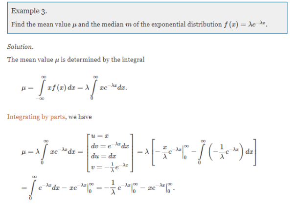
The mean value is μ=. The median of the exponential distribution is m =, and the variance is shown by .

Normal Distribution:

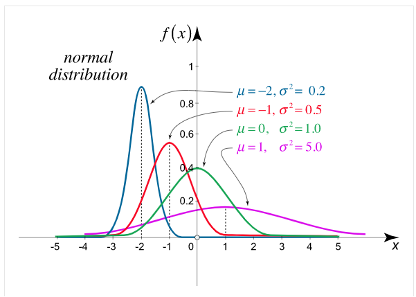
The normal distribution is the utmost broadly identified P.D. Then it defines many usual spectacles.

The PDF of the normal distribution is shown by method

f(x)= ,

Where μ is mean of the distribution, and is the variance.

The 2 limitations μ and σ completely describe the figure and all additional things of the normal distribution function.

Gamma density

Consider the distribution of the sum of 2 autonomous Exponential ( $\lambda$ ) R.V.

Density of the form:

$\begin{displaymath}f_S(s)=\int_0^s\lambda^2 e^{-\lambda s} dy= \lambda^2 s e^{-\lambda s} \end{displaymath}$

Density is knowm Gamma (2, density. In common the gamma density is precise with 2 reasons (t, as being non zero on the +ve reals and called:

$\begin{displaymath}f(x)=\frac{\lambda e^{-\lambda x} (\lambda x)^{t-1}}{\Gamma(t)}\end{displaymath}$

Where $\Gamma(t)$ is the endless which symbols integral of the density quantity to one:

$\begin{displaymath}\Gamma(t)=\int^{+\infty}_0 e^{-y} y^{t-1} dy\end{displaymath}$

By integration by parts we presented the significant recurrence relative:

$\begin{displaymath}\Gamma(t)=(t-1)\Gamma(t-1)\end{displaymath}$

Because $\Gamma(1)=\int_0^{+\infty}e^{-y}dy=1$ , we have for integer t=m

$\begin{displaymath}\Gamma(m)=(m-1)(m-2)\cdots \Gamma(1)=(m-1)!\end{displaymath}$

The specific case of the integer t can be linked to the sum of n independent exponential, it is the waiting time to the nth event, it is the matching of the negative binomial.

From that we can estimate what the estimated value and the variance are going to be: If all the Xi's are independent exponential (, then if we sum n of them we

Have $E(\sum_{1}^n X_i)=\frac{n}{\lambda}$ and if they are independent: $var(\sum_{1}^n X_i)=\frac{n}{\lambda^2}$

This simplifies to the non-integer t case:

$\begin{displaymath}E(X)=\frac{1}{\Gamma(t)} \int_0^{+\infty} \lambdax e^{-\lambd... ...da x)^t=\frac{\Gamma(t+1)}{\lambda\Gamma(t)}=\frac{t}{\lambda} \end{displaymath}$