Unit -4

Basic Statistics

4.1Measures of Central Tendency:

An mean is a value which is representative of a set of data. Average value may also be termed as measures of central tendency. There are five types of averages in common.

(i)Arithmetic average or mean

(ii) Median

(iii) Mode

(iv) Geometric Mean

(v) Harmonic Mean

ARITHMETIC MEAN:

(a)  If are n numbers, then their arithmetic mean (A.M.) is defined by

This is known as direct method.

(b)  Short cut method

Let a be the assumed mean, d the deviation of the variate x from a. Then

Example1. Find the arithmetic mean for the following distribution:

Solution.Let assumed mean (a) = 25

Class	Mid‐value	Frequency
40— 50
Total

(c) Step deviation method

Let be the assumed mean, the width ofthe class interval and

Example 2. Find the arithmetic mean of the data given in example 3 by step deviation method

Solution. Let

Class	Mid‐value	Frequency	a
Total

MEDIAN:

Median is defined as the measure of the central item when they are arranged in ascending or descending order ofmagnitude.

When the total number of the items is odd and equal to say , then the value of th item gives the median.

When the total number ofthe frequencies is even, say , then there are two middle items, and so the mean ofthe values of nth and th items is the median.

Example 3. Find the median of 6, 8, 9, 10, 11, 12, 13.

Solution. Total number of items

The middle item

Median Value of the 4th item

For grouped data, Median

Where is the lower limit of the median class, is the frequency of the class, is the width ofthe class‐interval, is the total ofall the preceeding frequencies of the median‐class and is total frequency ofthe data.

Example 4. Find the value ofMedian from the following data:

No. Of days for which absent (less than)
No. Of students

Solution. The given cumulative frequency distribution will first be converted into ordinary frequency as under

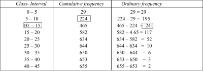
Median size of or 327.item

327.item lies in 10‐15 which is the median class.

Where stands for lower limit ofmedian class,

stands for the total frequency,

stands for the cumulative frequency just preceeding the median class, stands for class interval

stands for frequency for the median class.

Median

MODE

Mode is defined to be the size of the variable which occurs most frequently.

Example 5: Find the mode of the following items:

.

Solution. 6 occurs 5 times and no other item occurs 5 or more than 5 times, hence the mode is 6.

For grouped data,

Where is the lower limit of the modal class, is the frequency of the modal class, is the width of the class, is the frequency before the modal class and is the frequency after the modal class.

Emperical formula

Mean‐ Mode [Mean

Example 6. Find the mode from the following data:

	0—6	6—12	12—18		24—30	30—36

Solution.

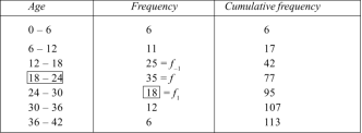
Mode

GEOMETRIC MEAN

, , be values of variates , then the geometric mean

Example 7. Find the geometric mean of 4, 8, 16.

Solution..

HARMONIC MEAN

Harmonic mean of a series of values is defined as the reciprocal of the arithmetic mean of their reciprocals. Thus be the harmonic mean, then

Example 8:Calculate the harmonic mean of 4, 8, 16.

Solution:

4.2 MOMENTS

The rth moment of a variable x about the mean x is usually denoted by is given by

The rth moment of a variable x aboutany point a is defined by

Relation between moments about mean and moment about any point:

where and

In particular

Note. 1. The sum ofthe coefficients ofthe various terms on the right‐hand side is zero.

2. The dimension of each term on right‐hand side is the same as that ofterms on the left.

MOMENT GENERATING FUNCTION

The moment generating function ofthe variate about is defined as the expected value of and is denoted .

Where , ‘ is the moment of order about

Hence coefficient of or

Again )

Thus the moment generating function about the point moment generating function about the origin.

SKEWNESS:

Skewness denotes the opposite of symmetry. It is lack of symmetry. In a symmetrical series, the mode, the median, and the arithmetic average are identical.

Coefficient of skewness

KURTOSIS: It measures the degree of peakedness of a distribution and is given by Measure of kurtosis.

Negative skewness      Positive skewness A.MesokurticB.Leptokurtic

C. Playkurtic

If , the curve is normal or mesokurtic.

If , the curve is peaked or leptokurtic.

If , the curve is flat topped or platykurtic

4.3 Probability Distributions: Binomial, Poisson and Normal

The Normal Distribution:

The normal distribution is sometimes informally called the bell curve.

The probability density of the normal distribution is:

 is mean or expectation of the distribution

 is the variance

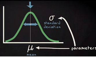
Properties of a normal distribution:

• The mean, mode and median are all equal.
• The curve is symmetric at the center (i.e. around the mean, μ).
• Exactly half of the values are to the left of center and exactly half the values are to the right.
• The total area under the curve is 1.

Binomial Distribution:

A distribution is said to be binomial distribution if the following conditions are met.

1. Each trial has a binary outcome (One of the two outcomes is labelled a ‘success’)
2. The probability of success is known and constant over all trials
3. The number of trials is specified
4. The trials are independent. That is, the outcome from one trial doesn’t affect the outcome of successive trials

If all the above conditions met then the binomial distribution describes the probability of X successes in n trials.

A classic example of the binomial distribution is the number of heads (X) in n coin tosses.

The Notation for a binomial distribution is

X ~ B (n, π)

Which is read as ‘X is distributed binomial with n trials and probability of success in one trial equal to π ’.

Formula for Binomial Distribution:

Using this formula, the probability distribution of a binomial random variable X can be calculated if n and π are known.

n! is called ‘n factorial’ = n(n-1)(n-2) . . .(1)

P(X) = #of Scenario * Single Scenario

The first factorial terms gives the number of scenario and the second term describes the probability of success to power of number of successes and probability of failure to the power of number of failures.

Poisson Distribution:

Another probability distribution for discrete variables is the Poisson distribution. The Poisson distribution is used to determine the probability of the number of events occurring over a specified time or space. This was named for Simeon D. Poisson, 1781 – 1840, French mathematician.

Examples of events over space or time: -number of cells in a specified volume of fluid

-number of calls/hour to a help line

-number of emergency room beds filled/ 24 hours

Like the binomial distribution and the normal distribution, there are many Poisson distributions.

• Each Poisson distribution is specified by the average rate at which the event occurs.
• The rate is notated with λ
• λ = ‘lambda’, Greek letter ‘L’ – There is only one parameter for the Poisson distribution

The probability that there are exactly X occurrences in the specified space or time is equal to

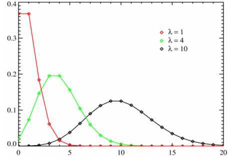
The horizontal axis is the index X. The function is defined only at integer values of X. The connecting lines are only guides for the eye and do not indicate continuity. Notice that as λ increases the distribution begins to resemble a normal distribution.

• If λ is 10 or greater, the normal distribution is a reasonable approximation to the Poisson distribution
• The mean and variance for a Poisson distribution are the same and are both equal to λ
• The standard deviation of the Poisson distribution is the square root of λ

4.4 Evaluation of Statistical Parameters for These Three Distributions

Normal Distribution Probability Calculation:

Probability density function or p.d.f. Specified the probability per unit of the random variable. Here is an example of a p.d.f. Of the daily waiting time by the taxi driver of Uber taxi company. In the X axis, daily waiting time and Y-axis probability per hour has been shown.

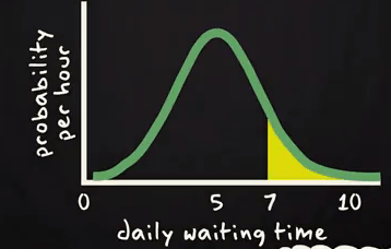
If one Uber taxi driver want to know the probability to wait more than 7 hours in a day? Then he will be interested in the yellow surface arear shown above. On basis of this graph you can estimate the area. Same thing you can get form below cumulative probability curve.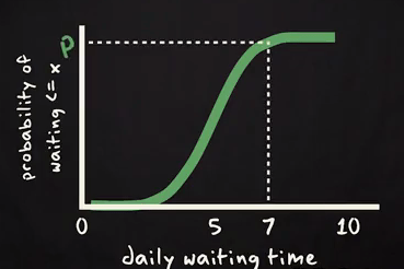

Probability to wait more than 7 hours will be calculated using complementary rule 1- P. Because corresponding to 7 in X axis we marked the probability is P and we are interested in more than 7 hours. So, P should be subtracted from 1 to get desired result.

Bell Shaped Distribution and Empirical Rule:

If distribution is bell shape then it is assumed that about 68% of the elements have a z-score between -1 and 1; about 95% have a z-score between -2 and 2; and about 99% have a z-score between -3 and 3.

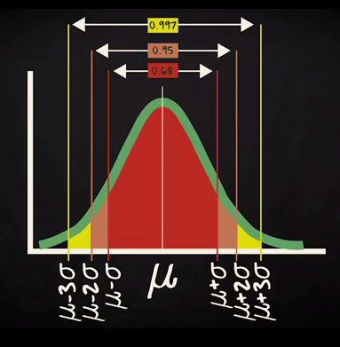
Assume the time you spend in week days by traveling has given by a normal distribution with mean= 40 mins and SD= 10 mins.

What will be your range of travel time for 95 % of your week days?

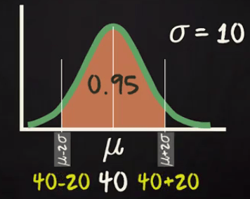
As you know 95 % will come within 2 standard deviation of your mean. So, the range will be (40-20) = 20 to (40+20) =60 mins.

Now another question you want to answer that what will be the probability to be travelling more than 50 mins?

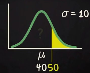
Actually you are interested in the yellow surface given in above diagram. You know that a normal distribution is symmetric. So, half of the probability located one side of the mean and another half located another side of the mean.

As SD =10. So, one standard deviation will be 30 to 50 range.

You already know for left side up 40 the probability is 0.5. Now if you calculate the probability from 40 to 50 range it will be half of 1 Standard deviation i.e.    0.68/2 = 0.34

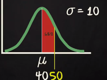
So the probability to travel less than 50 mins = 0.5 +. 0.34 = 0.84

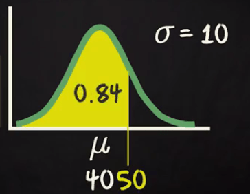
But you are interested in more than 50 mins traveling time so it will be 1- 0.84 =0.16

Binomial Distribution:

Example:

What is the probability of 2 heads in 6 coin tosses?

• Success = ‘heads’
• n = 6 trials
• π = 0.5
• X = number of heads in 6 tosses which is 2 here.
• X has a binomial distribution with n = 6 and π = 0.5
• X ~ B (6, 0.5)

So, probability of getting 2 heads is 0.234.

Consider another example:

In a sample of 8 patients with a heart attack, what is the probability that 2 patients will die if the probability of death from a heart attack = 0.03.

Assume that the probability of death is the same for all patients.

– Death from heart attack is a binary variable (Yes or No)

– ‘Success’ in this case is defined as death from heart attack

– n = number of ‘trials’ = 8 patients

– π = 0.03 = probability of success

– X = number of deaths. X =2 here.

X ~ B (8, 0.03)

If you follow the same formula you will get P(x=2) = 0.021

Poisson Distribution:

Example:

A large urban hospital has, on average, 80 emergency department admits every Monday. What is the probability that there will be more than 100?

If we put λ =80 and  x= 100 then we will get the probability value as 0.01316885.

To get the same result we can use normal approximation and then get the probability value.

Emergency room admits on a Monday?

• λ is the rate of admits / day on Monday = 80
• We can use the normal approximation since λ > 10

The normal approximation has mean = 80 and SD = 8.94 (the square root of 80 = 8.94)

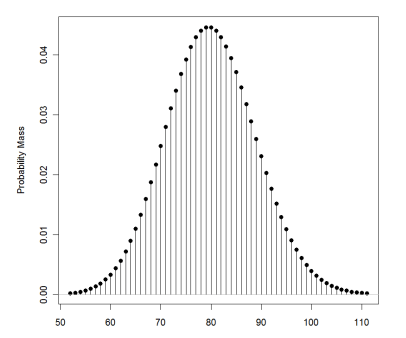
Now we can use the same way we calculate p-value for normal distribution. If you do that you will get a value of 0.01263871 which is very near to 0.01316885 what we get directly form Poisson formula. Here main intention is to show you how normal approximation works for Poisson Distribution.

4.5 CORRELATION

Whenever two variables x and y are so related that an increase in the one is accompanied by an increase or decrease in the other, then the variables are said to be correlated.

For example, the yield of crop varies with the amount of rainfall.

If an increase in one variable corresponds to an increase in the other, the correlation is said to be positive. If increase in one corresponds to the decrease in the other the correlation is said to be negative. If there is no relationship between the two variables, they are said to be independent.

Perfect Correlation: If two variables vary in such a way that their ratio is always constant, then the correlation is said to be perfect.

KARL PEARSON’S COEFFICIENT OF CORRELATION:

Rbetween two variables x and y is defined by the relation

Where,X = x –, Y = y –

i.e. X, Y are the deviations measured from their respective means,

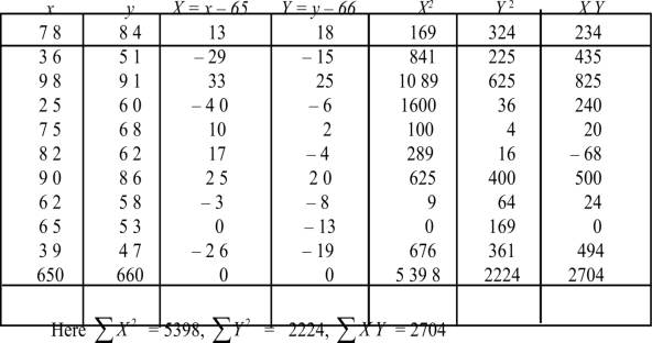
Example:Ten students got the following percentage of marks in Economics and Statistics

Calculate the of correlation.

Roll No.
Marks in Economics
Marks in

Solution:. Let the marks oftwo subjects be denoted by and respectively.

Then the mean for marks and the mean ofy marks

and are deviations ofx’s and ’s from their respective means, then the data may be arranged in the following form:

4.6 Spearman’s Rank Correlation

Solution. Let be the ranks of individuals corresponding to two characteristics.

Assuming nor two individuals are equal in either classification, each individual takes the values 1, 2, 3, and hence their arithmetic means are, each

Let , , , be the values of variable and , , those of

Then

Where and y are deviations from the mean.

Clearly, and

SPEARMAN’S RANK CORRELATION COEFFICIENT:

Where denotes rank coefficient of correlation and refers to the difference ofranks between paired items in two series.

Example:Compute Spearman’s rank correlation coefficient r for the following data:

Solution:

Person	Rank Statistics	Rank in income	d=
A	9	1	8	64
B	10	2	8	64
C	6	3	3	9
D	5	4	1	1
E	7	5	2	4
F	2	6	-4	16
G	4	7	-3	9
H	8	8	0	0
I	1	9	-8	64
J	3	10	-7	49

Example:IfXand Yare uncorrelated random variables, the of correlation between and

Solution.

Let and

Then

Now

Similarly

Now

Also

(As and are not correlated, we have )

Similarly

REGRESSION

Ifthe scatter diagram indicates some relationship between two variables and , then the dots of the scatter diagram will be concentrated round a curve. This curve is called the curve ofregression. Regression analysis is the method used for estimating the unknown values of one variable corresponding to the known value of another variable.

LINE OF REGRSSION

When the curve is a straight line, it is called a line of regression. A line of regression is the straight line which gives the best fit in the least square sense to the given frequency.

Example:Find the correlation betweenx and , when the lines ofregression are: and

Solution. Let the line of regression ofx on be

Then, the line ofregression ofy on is

And

which is not possible. So our choice of regression line is incorrect.

The regression line ofx on is

And, the regression line ofy on is

And

Hence the correlation coefficient between and is

Example: The following regression equations were obtainedfrom a correlation table:

Find the value of the correlation coefficient,

(b) the mean and

(c) the mean of

Solution.

(a)  From (1),

(b) From (2),

From (3) and (4)

Coefficient of correlation

(b) (1) and (2) pass through the point .

   (5)

   (6)

On solving (5) and (6), we get

References

1. E. Kreyszig, “Advanced Engineering Mathematics”, John Wiley & Sons, 2006.
2. P. G. Hoel, S. C. Port And C. J. Stone, “Introduction To Probability Theory”, Universal Book Stall, 2003.
3. S. Ross, “A First Course in Probability”, Pearson Education India, 2002.
4. W. Feller, “An Introduction To Probability Theory and Its Applications”, Vol. 1, Wiley, 1968.
5. N.P. Bali and M. Goyal, “A Text Book of Engineering Mathematics”, Laxmi Publications, 2010.
6. B.S. Grewal, “Higher Engineering Mathematics”, Khanna Publishers, 2000.
7. T. Veerarajan, “Engineering Mathematics”, Tata Mcgraw-Hill, New Delhi, 2010