Unit – 6

Classification and Prediction

6.1           What is classification and prediction

There are two forms of data analysis that can be used for extracting models describing important classes or to predict future data trends. These two forms are as follows −

• Classification
• Prediction

Classification models predict categorical class labels; and prediction models predict continuous valued functions. For example, we can build a classification model to categorize bank loan applications as either safe or risky, or a prediction model to predict the expenditures in dollars of potential customers on computer equipment given their income and occupation.

What is classification?

Following are the examples of cases where the data analysis task is Classification −

• A bank loan officer wants to analyze the data in order to know which customer (loan applicant) are risky or which are safe.
• A marketing manager at a company needs to analyze a customer with a given profile, who will buy a new computer.

In both of the above examples, a model or classifier is constructed to predict the categorical labels. These labels are risky or safe for loan application data and yes or no for marketing data.

What is prediction?

Following are the examples of cases where the data analysis task is Prediction −

Suppose the marketing manager needs to predict how much a given customer will spend during a sale at his company. In this example we are bothered to predict a numeric value. Therefore the data analysis task is an example of numeric prediction. In this case, a model or a predictor will be constructed that predicts a continuous-valued-function or ordered value.

Note − Regression analysis is a statistical methodology that is most often used for numeric prediction.

6.2           Issues regarding classification and prediction

1. Preparing the Data for Classification and Prediction

The following preprocessing steps may be applied to the data in order to help improve the accuracy, efficiency, and scalability of the classification or prediction process.

Data Cleaning: This refers to the preprocessing of data in order to remove or reduce noise (by applying smoothing techniques) and the treatment of missing values (e.g., by replacing a missing value with the most commonly occurring value for that attribute, or with the most probable value based on statistics.) Although most classification algorithms have some mechanisms for handling noisy or missing data, this step can help reduce confusion during learning.

Relevance Analysis: Many of the attributes in the data may be irrelevant to the classification or prediction task. For example, data recording the day of the week on which a bank loan application was filed is unlikely to be relevant to the success of the application. Furthermore, other attributes may be redundant. Hence, relevance analysis may be performed on the data with the aim of removing any irrelevant or redundant attributes from the learning process. In machine learning, this step is known as feature selection. Including such attributes may otherwise slow down, and possibly mislead, the learning step.

Ideally, the time spent on relevance analysis, when added to the time spent on learning from the resulting “reduced” feature subset should be less than the time that would have been spent on learning from the original set of features. Hence, such analysis can help improve classification efficiency and scalability.

Data Transformation: The data can be generalized to higher – level concepts. Concept hierarchies may be used for this purpose. This is particularly useful for continuous – valued attributes. For example, numeric values for the attribute income may be generalized to discrete ranges such as low, medium, and high. Similarly, nominal – valued attributes like street, can be generalized to higher – level concepts, like city. Since generalization compresses the original training data, fewer input / output operations may be involved during learning.

The data may also be normalized, particularly when neural networks or methods involving distance measurements are used in the learning step. Normalization involves scaling all values for a given attribute so that they fall within a small specified range, such as – 1.0 to 1.0, or 0.0 to 1.0. In methods that use distance measurements, for example, this would prevent attributes with initially large ranges (like, say, income) from outweighing attributes with initially smaller ranges (such as binary attributes).

2. Comparing Classification Methods

Classification and prediction methods can be compared and evaluated according to the following criteria:

Predictive Accuracy: This refers to the ability of the model to correctly predict the class label of new or previously unseen data.

Speed: This refers to the computation costs involved in generating and using the model.

Robustness: This is the ability of the model to make correct predictions given noisy data or data with missing values.

Scalability: This refers to the ability to construct the model efficiently given large amount of data.

Interpretability: This refers to the level of understanding and insight that is provided by the model.

6.3           Classification by decision tree Induction

Decision Tree Mining is a type of data mining technique that is used to build Classification Models. It builds classification models in the form of a tree-like structure, just like its name. This type of mining belongs to supervised class learning.

In supervised learning, the target result is already known. Decision trees can be used for both categorical and numerical data. The categorical data represent gender, marital status, etc. while the numerical data represent age, temperature, etc.

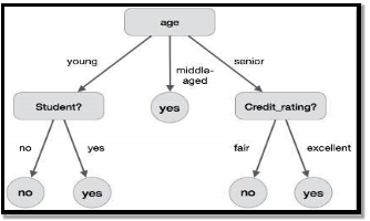
A decision tree is a structure that includes a root node, branches, and leaf nodes. Each internal node denotes a test on an attribute, each branch denotes the outcome of a test, and each leaf node holds a class label. The topmost node in the tree is the root node.

The following decision tree is for the concept buy_computer that indicates whether a customer at a company is likely to buy a computer or not. Each internal node represents a test on an attribute. Each leaf node represents a class.

The benefits of having a decision tree are as follows −

• It does not require any domain knowledge.
• It is easy to comprehend.
• The learning and classification steps of a decision tree are simple and fast.

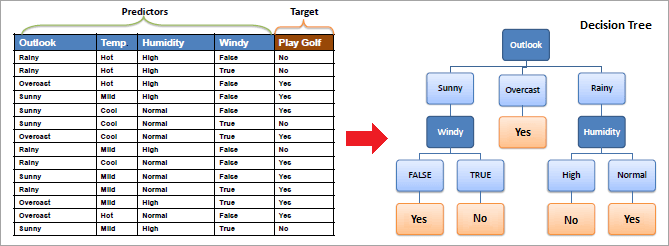
An example of a decision tree with the dataset is shown below.

What Is The Use Of A Decision Tree?

Decision Tree is used to build classification and regression models. It is used to create data models that will predict class labels or values for the decision-making process. The models are built from the training dataset fed to the system (supervised learning).

Using a decision tree, we can visualize the decisions that make it easy to understand and thus it is a popular data mining technique.

Classification Analysis

Data Classification is a form of analysis which builds a model that describes important class variables. For example, a model built to categorize bank loan applications as safe or risky. Classification methods are used in machine learning, and pattern recognition.

Application of classification includes fraud detection, medical diagnosis, target marketing, etc. The output of the classification problem is taken as “Mode” of all observed values of the terminal node.

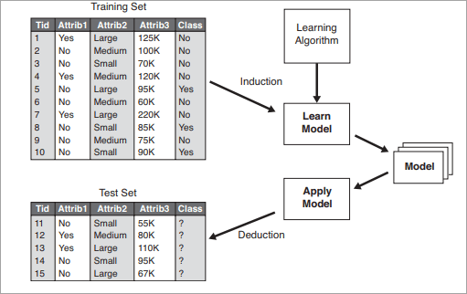
A two-step process is followed, to build a classification model.

1. In the first step i.e. learning: A classification model based on training data is built.
2. In the second step i.e. Classification, the accuracy of the model is checked and then the model is used to classify new data. The class labels presented here are in the form of discrete values such as “yes” or “no”, “safe” or “risky”.

The general approach for building classification models is given below:

Regression Analysis

Regression analysis is used for the prediction of numeric attributes.

Numeric attributes are also called continuous values. A model built to predict the continuous values instead of class labels is called the regression model. The output of regression analysis is the “Mean” of all observed values of the node.

How Does A Decision Tree Work?

A decision tree is a supervised learning algorithm that works for both discrete and continuous variables. It splits the dataset into subsets on the basis of the most significant attribute in the dataset. How the decision tree identifies this attribute and how this splitting is done is decided by the algorithms.

The most significant predictor is designated as the root node, splitting is done to form sub-nodes called decision nodes, and the nodes which do not split further are terminal or leaf nodes.

In the decision tree, the dataset is divided into homogeneous and non-overlapping regions. It follows a top-down approach as the top region presents all the observations at a single place which splits into two or more branches that further split. This approach is also called a greedy approach as it only considers the current node between the worked on without focusing on the future nodes.

The decision tree algorithms will continue running until a stop criteria such as the minimum number of observations etc. is reached.Once a decision tree is built, many nodes may represent outliers or noisy data. Tree pruning method is applied to remove unwanted data. This, in turn, improves the accuracy of the classification model.

To find the accuracy of the model, a test set consisting of test tuples and class labels is used. The percentages of the test set tuples are correctly classified by the model to identify the accuracy of the model. If the model is found to be accurate then it is used to classify the data tuples for which the class labels are not known.

Some of the decision tree algorithms include Hunt’s Algorithm, ID3, CD4.5, and CART.

Example of Creating a Decision Tree

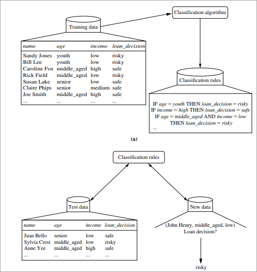
(Example is taken from Data Mining Concepts: Han and Kimber)

#1) Learning Step: The training data is fed into the system to be analyzed by a classification algorithm. In this example, the class label is the attribute i.e. “loan decision”. The model built from this training data is represented in the form of decision rules.

#2) Classification: Test dataset are fed to the model to check the accuracy of the classification rule. If the model gives acceptable results then it is applied to a new dataset with unknown class variables.

Decision Tree Induction Algorithm

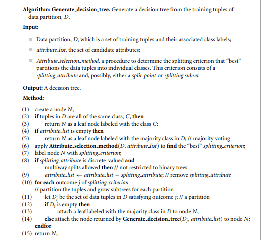
Decision Tree Induction

Decision tree induction is the method of learning the decision trees from the training set. The training set consists of attributes and class labels. Applications of decision tree induction include astronomy, financial analysis, medical diagnosis, manufacturing, and production.

A decision tree is a flowchart tree-like structure that is made from training set tuples. The dataset is broken down into smaller subsets and is present in the form of nodes of a tree. The tree structure has a root node, internal nodes or decision nodes, leaf node, and branches.

The root node is the topmost node. It represents the best attribute selected for classification. Internal nodes of the decision nodes represent a test of an attribute of the dataset leaf node or terminal node which represents the classification or decision label. The branches show the outcome of the test performed.

Some decision trees only have binary nodes, that means exactly two branches of a node, while some decision trees are non-binary.

The image below shows the decision tree for the Titanic dataset to predict whether the passenger will survive or not.

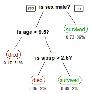
CART

CART model i.e. Classification and Regression Models is a decision tree algorithm for building models. Decision Tree model where the target values have a discrete nature is called classification models.

A discrete value is a finite or countably infinite set of values, For Example, age, size, etc. The models where the target values are represented by continuous values are usually numbers that are called Regression Models. Continuous variables are floating-point variables. These two models together are called CART.

CART uses Gini Index as Classification matrix.

Decision Tree Induction for Machine Learning: ID3

In the late 1970s and early 1980s, J.Ross Quinlan was a researcher who built a decision tree algorithm for machine learning. This algorithm is known as ID3, Iterative Dichotomiser. This algorithm was an extension of the concept learning systems described by E.B Hunt, J, and Marin.

ID3 later came to be known as C4.5. ID3 and C4.5 follow a greedy top-down approach for constructing decision trees. The algorithm starts with a training dataset with class labels that are portioned into smaller subsets as the tree is being constructed.

#1) Initially, there are three parameters i.e. attribute list, attribute selection method and data partition. The attribute list describes the attributes of the training set tuples.

#2) The attribute selection method describes the method for selecting the best attribute for discrimination among tuples. The methods used for attribute selection can either be Information Gain or Gini Index.

#3) The structure of the tree (binary or non-binary) is decided by the attribute selection method.

#4) When constructing a decision tree, it starts as a single node representing the tuples.

#5) If the root node tuples represent different class labels, then it calls an attribute selection method to split or partition the tuples. The step will lead to the formation of branches and decision nodes.

#6) The splitting method will determine which attribute should be selected to partition the data tuples. It also determines the branches to be grown from the node according to the test outcome. The main motive of the splitting criteria is that the partition at each branch of the decision tree should represent the same class label.

An example of splitting attribute is shown below:

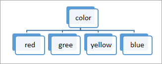
a. The portioning above is discrete-valued.

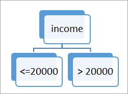
b. The portioning above is for continuous-valued.

#7) The above partitioning steps are followed recursively to form a decision tree for the training dataset tuples.

#8) The portioning stops only when either all the partitions are made or when the remaining tuples cannot be partitioned further.

#9) The complexity of the algorithm is described by n * |D| * log |D| where n is the number of attributes in training dataset D and |D| is the number of tuples.

What Is Greedy Recursive Binary Splitting?

In the binary splitting method, the tuples are split and each split cost function is calculated. The lowest cost split is selected. The splitting method is binary which is formed as 2 branches. It is recursive in nature as the same method (calculating the cost) is used for splitting the other tuples of the dataset.

This algorithm is called as greedy as it focuses only on the current node. It focuses on lowering its cost, while the other nodes are ignored.

How To Select Attributes For Creating A Tree?

Attribute selection measures are also called splitting rules to decide how the tuples are going to split. The splitting criteria are used to best partition the dataset. These measures provide a ranking to the attributes for partitioning the training tuples.

The most popular methods of selecting the attribute are information gain, Gini index.

#1) Information Gain

This method is the main method that is used to build decision trees. It reduces the information that is required to classify the tuples. It reduces the number of tests that are needed to classify the given tuple. The attribute with the highest information gain is selected.

The original information needed for classification of a tuple in dataset D is given by:

Where p is the probability that the tuple belongs to class C. The information is encoded in bits, therefore, log to the base 2 is used. E(s) represents the average amount of information required to find out the class label of dataset D. This information gain is also called Entropy.

The information required for exact classification after portioning is given by the formula:

Where P (c) is the weight of partition. This information represents the information needed to classify the dataset D on portioning by X.

Information gain is the difference between the original and expected information that is required to classify the tuples of dataset D.

Gain is the reduction of information that is required by knowing the value of X. The attribute with the highest information gain is chosen as “best”.

#2) Gain Ratio

Information gain might sometimes result in portioning useless for classification. However, the Gain ratio splits the training data set into partitions and considers the number of tuples of the outcome with respect to the total tuples. The attribute with the max gain ratio is used as a splitting attribute.

#3) Gini Index

Gini Index is calculated for binary variables only. It measures the impurity in training tuples of dataset D, as

P is the probability that tuple belongs to class C. The Gini index that is calculated for binary split dataset D by attribute A is given by:

Where n is the nth partition of the dataset D.

The reduction in impurity is given by the difference of the Gini index of the original dataset D and Gini index after partition by attribute A.

The maximum reduction in impurity or max Gini index is selected as the best attribute for splitting.

Overfitting In Decision Trees

Overfitting happens when a decision tree tries to be as perfect as possible by increasing the depth of tests and thereby reduces the error. This results in very complex trees and leads to overfitting.

Overfitting reduces the predictive nature of the decision tree. The approaches to avoid overfitting of the trees include pre pruning and post pruning.

What Is Tree Pruning?

Pruning is the method of removing the unused branches from the decision tree. Some branches of the decision tree might represent outliers or noisy data.

Tree pruning is the method to reduce the unwanted branches of the tree. This will reduce the complexity of the tree and help in effective predictive analysis. It reduces the overfitting as it removes the unimportant branches from the trees.

There are two ways of pruning the tree:

#1) Prepruning: In this approach, the construction of the decision tree is stopped early. It

Means it is decided not to further partition the branches. The last node constructed becomes the leaf node and this leaf node may hold the most frequent class among the tuples.

The attribute selection measures are used to find out the weightage of the split. Threshold values are prescribed to decide which splits are regarded as useful. If the portioning of the node results in splitting by falling below threshold then the process is halted.

#2) Post pruning: This method removes the outlier branches from a fully grown tree. The unwanted branches are removed and replaced by a leaf node denoting the most frequent class label. This technique requires more computation than prepruning, however, it is more reliable.

The pruned trees are more precise and compact when compared to unpruned trees but they carry a disadvantage of replication and repetition.

Repetition occurs when the same attribute is tested again and again along a branch of a tree. Replication occurs when the duplicate subtrees are present within the tree. These issues can be solved by multivariate splits.

The Below image shows an unpruned and pruned tree.

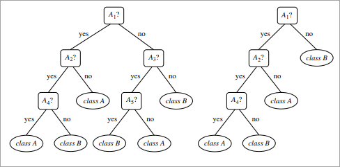
Example of Decision Tree Algorithm

Constructing a Decision Tree

Let us take an example of the last 10 days weather dataset with attributes outlook, temperature, wind, and humidity. The outcome variable will be playing cricket or not. We will use the ID3 algorithm to build the decision tree.

Step1: The first step will be to create a root node.

Step2: If all results are yes, then the leaf node “yes” will be returned else the leaf node “no” will be returned.

Step3: Find out the Entropy of all observations and entropy with attribute “x” that is E(S) and E(S, x).

Step4: Find out the information gain and select the attribute with high information gain.

Step5: Repeat the above steps until all attributes are covered.

Calculation of Entropy:

Yes                           No

9                                5

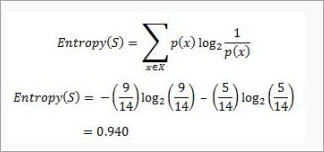
If entropy is zero, it means that all members belong to the same class and if entropy is one then it means that half of the tuples belong to one class and one of them belong to other class. 0.94 means fair distribution.

Find the information gain attribute which gives maximum information gain.

For Example “Wind”, it takes two values: Strong and Weak, therefore, x = {Strong, Weak}.

Find out H(x), P(x) for x =weak and x= strong. H(S) is already calculated above.

Weak= 8

Strong= 8

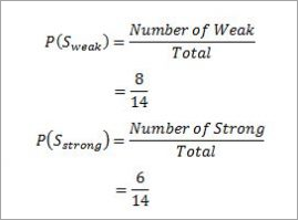
For “weak” wind, 6 of them say “Yes” to play cricket and 2 of them say “No”. So entropy will be:

For “strong” wind, 3 said “No” to play cricket and 3 said “Yes”. 

This shows perfect randomness as half items belong to one class and the remaining half belong to others.

Calculate the information gain,

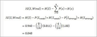
Similarly the information gain for other attributes is:

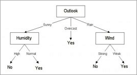
The attribute outlook has the highest information gain of 0.246, thus it is chosen as root.

Overcast has 3 values: Sunny, Overcast and Rain. Overcast with play cricket is always “Yes”. So it ends up with a leaf node, “yes”. For the other values “Sunny” and “Rain”.

Table for Outlook as “Sunny” will be:

Entropy for “Outlook” “Sunny” is:

Information gain for attributes with respect to Sunny is:

The information gain for humidity is highest, therefore it is chosen as the next node. Similarly, Entropy is calculated for Rain. Wind gives the highest information gain.

The decision tree would look like below:

What Is Predictive Modelling?

The classification models can be used to predict the outcomes of an unknown set of attributes.

When a dataset with unknown class labels is fed into the model, then it will automatically assign the class label to it. This method of applying probability to predict outcomes is called predictive modeling.

Advantages Of Decision Tree Classification

Enlisted below are the various merits of Decision Tree Classification:

1. Decision tree classification does not require any domain knowledge, hence, it is appropriate for the knowledge discovery process.
2. The representation of data in the form of the tree is easily understood by humans and it is intuitive.
3. It can handle multidimensional data.
4. It is a quick process with great accuracy.

Disadvantages Of Decision Tree Classification

Given below are the various demerits of Decision Tree Classification:

1. Sometimes decision trees become very complex and these are called overfitted trees.
2. The decision tree algorithm may not be an optimal solution.
3. The decision trees may return a biased solution if some class label dominates it.

Conclusion

Decision Trees are data mining techniques for classification and regression analysis.

This technique is now spanning over many areas like medical diagnosis, target marketing, etc. These trees are constructed by following an algorithm such as ID3, CART. These algorithms find different ways to split the data into partitions.

It is the most widely known supervised learning technique that is used in machine learning and pattern analysis. The decision trees predict the values of the target variable by building models through learning from the training set provided to the system.

6.4           Bayesian Classification

This article discusses the theory behind the Naive Bayes classifiers and their implementation.

Naive Bayes classifiers are a collection of classification algorithms based on Bayes’ Theorem. It is not a single algorithm but a family of algorithms where all of them share a common principle, i.e. every pair of features being classified is independent of each other.

To start with, let us consider a dataset.

Consider a fictional dataset that describes the weather conditions for playing a game of golf. Given the weather conditions, each tuple classifies the conditions as fit(“Yes”) or unfit(“No”) for plaing golf.

Here is a tabular representation of our dataset.

The dataset is divided into two parts, namely, feature matrix and the response vector.

• Feature matrix contains all the vectors(rows) of dataset in which each vector consists of the value of dependent features. In above dataset, features are ‘Outlook’, ‘Temperature’, ‘Humidity’ and ‘Windy’.
• Response vector contains the value of class variable(prediction or output) for each row of feature matrix. In above dataset, the class variable name is ‘Play golf’.

Assumption:

The fundamental Naive Bayes assumption is that each feature makes an:

• Independent
• Equal

Contribution to the outcome.

With relation to our dataset, this concept can be understood as:

• We assume that no pair of features are dependent. For example, the temperature being ‘Hot’ has nothing to do with the humidity or the outlook being ‘Rainy’ has no effect on the winds. Hence, the features are assumed to be independent.
• Secondly, each feature is given the same weight(or importance). For example, knowing only temperature and humidity alone can’t predict the outcome accuratey. None of the attributes is irrelevant and assumed to be contributing equally to the outcome.

Note: The assumptions made by Naive Bayes are not generally correct in real-world situations. In-fact, the independence assumption is never correct but often works well in practice.

Now, before moving to the formula for Naive Bayes, it is important to know about Bayes’ theorem.

Bayes’ Theorem finds the probability of an event occurring given the probability of another event that has already occurred. Bayes’ theorem is stated mathematically as the following equation:

Where A and B are events and P(B) ? 0.

• Basically, we are trying to find probability of event A, given the event B is true. Event B is also termed as evidence.
• P(A) is the priori of A (the prior probability, i.e. Probability of event before evidence is seen). The evidence is an attribute value of an unknown instance(here, it is event B).
• P(A|B) is a posteriori probability of B, i.e. probability of event after evidence is seen.

Now, with regards to our dataset, we can apply Bayes’ theorem in following way:

Where, y is class variable and X is a dependent feature vector (of size n) where:

Just to clear, an example of a feature vector and corresponding class variable can be: (refer 1st row of dataset)

X = (Rainy, Hot, High, False)

y = No

So basically, P(X|y) here means, the probability of “Not playing golf” given that the weather conditions are “Rainy outlook”, “Temperature is hot”, “high humidity” and “no wind”.

Now, its time to put a naive assumption to the Bayes’ theorem, which is, independence among the features. So now, we split evidence into the independent parts.

Now, if any two events A and B are independent, then,

P(A,B) = P(A)P(B)

Hence, we reach to the result:

Which can be expressed as:

Now, as the denominator remains constant for a given input, we can remove that term:

Now, we need to create a classifier model. For this, we find the probability of given set of inputs for all possible values of the class variable y and pick up the output with maximum probability. This can be expressed mathematically as:

So, finally, we are left with the task of calculating P(y) and P(xi | y).

Please note that P(y) is also called class probability and P(xi | y) is called conditional probability.

The different naive Bayes classifiers differ mainly by the assumptions they make regarding the distribution of P(xi | y).

Let us try to apply the above formula manually on our weather dataset. For this, we need to do some precomputations on our dataset.

We need to find P(xi | yj) for each xi in X and yj in y. All these calculations have been demonstrated in the tables below:

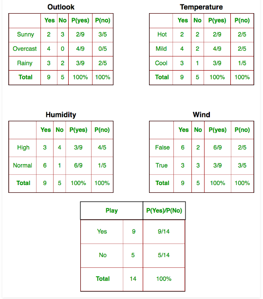
So, in the figure above, we have calculated P(xi | yj) for each xi in X and yj in y manually in the tables 1-4. For example, probability of playing golf given that the temperature is cool, i.eP(temp. = cool | play golf = Yes) = 3/9.

Also, we need to find class probabilities (P(y)) which has been calculated in the table 5. For example, P(play golf = Yes) = 9/14.

So now, we are done with our pre-computations and the classifier is ready!

Let us test it on a new set of features (let us call it today):

Today = (Sunny, Hot, Normal, False)

So, probability of playing golf is given by:

And probability to not play golf is given by:

Since, P(today) is common in both probabilities, we can ignore P(today) and find proportional probabilities as:

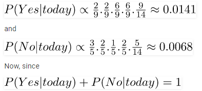
These numbers can be converted into a probability by making the sum equal to 1 (normalization):

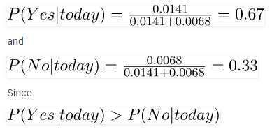
So, prediction that golf would be played is ‘Yes’.

The method that we discussed above is applicable for discrete data. In case of continuous data, we need to make some assumptions regarding the distribution of values of each feature. The different naive Bayes classifiers differ mainly by the assumptions they make regarding the distribution of P(xi | y).

6.5           Classification based on concepts from association rule mining

Association rule mining finds patterns in data.In other words interesting associations and relationships among large sets of data items can be done using association rules. This rule shows how likely a item set occurs in a transaction. A typical example is Market Based Analysis.

Market Based Analysis allows retailers to identify relationships between the items that people buy together frequently .Through a given a set of transactions, we can find rules that will predict the frequency of an item based on the occurrences of other items in the transaction.

Some of the basic definitions include:

Support Count (σ) – Frequency of occurrence of a item set.

Here σ ({Milk, Bread, Diaper}) =2

Frequent Item set – An item set whose support is greater than or equal to min sup threshold.

Association Rule – An implication expression of the form X -> Y, where X and Y are any 2 item sets.

Example: {Milk, Diaper} -> {Beer}

Rule Evaluation Metrics –

• Support(s) :
  The number of transactions that include items in the {X} and {Y} parts of the rule as a percentage of the total number of transaction. It is a measure of how frequently the collection of items occur together as a percentage of all transactions.
• Support = σ (X+Y) ÷ total :
  It is interpreted as fraction of transactions that contain both X and Y.
• Confidence(c) :
  It is the ratio of the no of transactions that includes all items in {B} as well as the no of transactions that includes all items in {A} to the no of transactions that includes all items in {A}.

• Conf(X=>Y) = Supp(X U Y) ÷ Supp(X) :
  It measures how often each item in Y appears in transactions that contains items in X also.
• Lift(l) :
  The lift of the rule X=>Y is the confidence of the rule divided by the expected confidence, assuming that the itemsets X and Y are independent of each other.The expected confidence is the confidence divided by the frequency of {Y}.
• Lift(X=>Y) = Conf(X=>Y) ÷ Supp(Y) :
  Lift value near 1 indicates X and Y almost often appear together as expected, greater than 1 means they appear together more than expected and less than 1 means they appear less than expected.Greater lift values indicate stronger association.

Example – From the above table, {Milk, Diaper}=>{Beer}

s= ({Milk, Diaper, Beer}) ÷ |T|

= 2/5

= 0.4

c= (Milk, Diaper, Beer) ÷ σ (Milk, Diaper)

= 2/3

= 0.67

l= Supp({Milk, Diaper, Beer}) ÷ Supp({Milk, Diaper})*Supp({Beer})

= 0.4/(0.6*0.6)

= 1.11

6.6           Prediction

Following are the examples of cases where the data analysis task is Prediction −

Suppose the marketing manager needs to predict how much a given customer will spend during a sale at his company. In this example we are bothered to predict a numeric value. Therefore the data analysis task is an example of numeric prediction. In this case, a model or a predictor will be constructed that predicts a continuous-valued-function or ordered value.

Note − Regression analysis is a statistical methodology that is most often used for numeric prediction.

6.7           Classification accuracy

Accuracy is one metric for evaluating classification models. Informally, accuracy is the fraction of predictions our model got right. Formally, accuracy has the following definition:

Accuracy=Number of correct predictions / Total number of predictions

For binary classification, accuracy can also be calculated in terms of positives and negatives as follows:

Accuracy=TP+TNTP+TN+FP+FN

Where TP = True Positives, TN = True Negatives, FP = False Positives, and FN = False Negatives.

Reference Books

1        Data Mining : Next Generation Challenges and Future Direction by Kargupta, et al, PHI.

2        Data Warehousing, Data Mining & OLAP by Alex Berson Stephen J.Smith.