UNIT 1
Introduction
What is Artificial Intelligence?
In today's world, technology is growing very fast, and we are getting in touch with different new technologies day by day.
Here, one of the booming technologies of computer science is Artificial Intelligence which is ready to create a new revolution in the world by making intelligent machines.The Artificial Intelligence is now all around us. It is currently working with a variety of subfields, ranging from general to specific, such as self-driving cars, playing chess, proving theorems, playing music, Painting, etc.
AI is one of the fascinating and universal fields of Computer science which has a great scope in future. AI holds a tendency to cause a machine to work as a human.

Artificial Intelligence is composed of two words Artificial and Intelligence, where Artificial defines "man-made," and intelligence defines "thinking power", hence AI means "a man-made thinking power."
So, we can define AI as:
"It is a branch of computer science by which we can create intelligent machines which can behave like a human, think like humans, and able to make decisions."
Artificial Intelligence exists when a machine can have human based skills such as learning, reasoning, and solving problems
With Artificial Intelligence you do not need to preprogram a machine to do some work, despite that you can create a machine with programmed algorithms which can work with own intelligence, and that is the awesomeness of AI.
It is believed that AI is not a new technology, and some people says that as per Greek myth, there were Mechanical men in early days which can work and behave like humans.
Why Artificial Intelligence?
Before Learning about Artificial Intelligence, we should know that what is the importance of AI and why should we learn it. Following are some main reasons to learn about AI:
- With the help of AI, you can create such software or devices which can solve real-world problems very easily and with accuracy such as health issues, marketing, traffic issues, etc.
- With the help of AI, you can create your personal virtual Assistant, such as Cortana, Google Assistant, Siri, etc.
- With the help of AI, you can build such Robots which can work in an environment where survival of humans can be at risk.
- AI opens a path for other new technologies, new devices, and new Opportunities.
Goals of Artificial Intelligence
Following are the main goals of Artificial Intelligence:
- Replicate human intelligence
- Solve Knowledge-intensive tasks
- An intelligent connection of perception and action
- Building a machine which can perform tasks that requires human intelligence such as:
- Proving a theorem
- Playing chess
- Plan some surgical operation
- Driving a car in traffic
- Creating some system which can exhibit intelligent behavior, learn new things by itself, demonstrate, explain, and can advise to its user.
What Comprises to Artificial Intelligence?
Artificial Intelligence is not just a part of computer science even it's so vast and requires lots of other factors which can contribute to it. To create the AI first we should know that how intelligence is composed, so the Intelligence is an intangible part of our brain which is a combination of Reasoning, learning, problem-solving perception, language understanding, etc.
To achieve the above factors for a machine or software Artificial Intelligence requires the following discipline:
- Mathematics
- Biology
- Psychology
- Sociology
- Computer Science
- Neurons Study
- Statistics

Advantages of Artificial Intelligence
Following are some main advantages of Artificial Intelligence:
- High Accuracy with less errors: AI machines or systems are prone to less errors and high accuracy as it takes decisions as per pre-experience or information.
- High-Speed: AI systems can be of very high-speed and fast-decision making, because of that AI systems can beat a chess champion in the Chess game.
- High reliability: AI machines are highly reliable and can perform the same action multiple times with high accuracy.
- Useful for risky areas: AI machines can be helpful in situations such as defusing a bomb, exploring the ocean floor, where to employ a human can be risky.
- Digital Assistant: AI can be very useful to provide digital assistant to the users such as AI technology is currently used by various E-commerce websites to show the products as per customer requirement.
- Useful as a public utility: AI can be very useful for public utilities such as a self-driving car which can make our journey safer and hassle-free, facial recognition for security purpose, Natural language processing to communicate with the human in human-language, etc.
Disadvantages of Artificial Intelligence
Every technology has some disadvantages, and thesame goes for Artificial intelligence. Being so advantageous technology still, it has some disadvantages which we need to keep in our mind while creating an AI system. Following are the disadvantages of AI:
- High Cost: The hardware and software requirement of AI is very costly as it requires lots of maintenance to meet current world requirements.
- Can't think out of the box: Even we are making smarter machines with AI, but still they cannot work out of the box, as the robot will only do that work for which they are trained, or programmed.
- No feelings and emotions: AI machines can be an outstanding performer, but still it does not have the feeling so it cannot make any kind of emotional attachment with human, and may sometime be harmful for users if the proper care is not taken.
- Increase dependency on machines: With the increment of technology, people are getting more dependent on devices and hence they are losing their mental capabilities.
- No Original Creativity: As humans are so creative and can imagine some new ideas but still AI machines cannot beat this power of human intelligence and cannot be creative and imaginative.
In 1950, Alan Turing introduced a test to check whether a machine can think like a human or not, this test is known as the Turing Test. In this test, Turing proposed that the computer can be said to be an intelligent if it can mimic human response under specific conditions.
Turing Test was introduced by Turing in his 1950 paper, "Computing Machinery and Intelligence," which considered the question, "Can Machine think?"
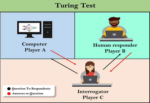
The Turing test is based on a party game "Imitation game," with some modifications. This game involves three players in which one player is Computer, another player is human responder, and the third player is a human Interrogator, who is isolated from other two players and his job is to find that which player is machine among two of them.
Consider, Player A is a computer, Player B is human, and Player C is an interrogator. Interrogator is aware that one of them is machine, but he needs to identify this on the basis of questions and their responses.
The conversation between all players is via keyboard and screen so the result would not depend on the machine's ability to convert words as speech.
The test result does not depend on each correct answer, but only how closely its responses like a human answer. The computer is permitted to do everything possible to force a wrong identification by the interrogator.
The questions and answers can be like:
Interrogator: Are you a computer?
PlayerA (Computer): No
Interrogator: Multiply two large numbers such as (256896489*456725896)
Player A: Long pause and give the wrong answer.
In this game, if an interrogator would not be able to identify which is a machine and which is human, then the computer passes the test successfully, and the machine is said to be intelligent and can think like a human.
"In 1991, the New York businessman Hugh Loebner announces the prize competition, offering a $100,000 prize for the first computer to pass the Turing test. However, no AI program to till date, come close to passing an undiluted Turing test".
Chatbots to attempt the Turing test:
ELIZA: ELIZA was a Natural language processing computer program created by Joseph Weizenbaum. It was created to demonstrate the ability of communication between machine and humans. It was one of the first chatterbots, which has attempted the Turing Test.
Parry: Parry was a chatterbot created by Kenneth Colby in 1972. Parry was designed to simulate a person with Paranoid schizophrenia(most common chronic mental disorder). Parry was described as "ELIZA with attitude." Parry was tested using a variation of the Turing Test in the early 1970s.
Eugene Goostman: Eugene Goostman was a chatbot developed in Saint Petersburg in 2001. This bot has competed in the various number of Turing Test. In June 2012, at an event, Goostman won the competition promoted as largest-ever Turing test content, in which it has convinced 29% of judges that it was a human.Goostman resembled as a 13-year old virtual boy.
The Chinese Room Argument:
There were many philosophers who really disagreed with the complete concept of Artificial Intelligence. The most famous argument in this list was "Chinese Room."
In the year 1980, John Searle presented "Chinese Room" thought experiment, in his paper "Mind, Brains, and Program," which was against the validity of Turing's Test. According to his argument, "Programming a computer may make it to understand a language, but it will not produce a real understanding of language or consciousness in a computer."
He argued that Machine such as ELIZA and Parry could easily pass the Turing test by manipulating keywords and symbol, but they had no real understanding of language. So it cannot be described as "thinking" capability of a machine such as a human.
Features required for a machine to pass the Turing test:
- Natural language processing: NLP is required to communicate with Interrogator in general human language like English.
- Knowledge representation: To store and retrieve information during the test.
- Automated reasoning: To use the previously stored information for answering the questions.
- Machine learning: To adapt new changes and can detect generalized patterns.
- Vision (For total Turing test): To recognize the interrogator actions and other objects during a test.
- Motor Control (For total Turing test): To act upon objects if requested.
Agents in Artificial Intelligence
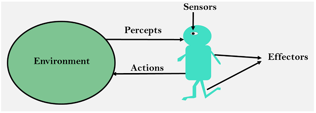
An AI system can be defined as the study of the rational agent and its environment. The agents sense the environment through sensors and act on their environment through actuators. An AI agent can have mental properties such as knowledge, belief, intention, etc.
What is an Agent?
An agent can be anything that perceiveits environment through sensors and act upon that environment through actuators. An Agent runs in the cycle of perceiving, thinking, and acting. An agent can be:
- Human-Agent: A human agent has eyes, ears, and other organs which work for sensors and hand, legs, vocal tract work for actuators.
- Robotic Agent: A robotic agent can have cameras, infrared range finder, NLP for sensors and various motors for actuators.
- Software Agent: Software agent can have keystrokes, file contents as sensory input and act on those inputs and display output on the screen.
Hence the world around us is full of agents such as thermostat, cellphone, camera, and even we are also agents.
Before moving forward, we should first know about sensors, effectors, and actuators.
Sensor: Sensor is a device which detects the change in the environment and sends the information to other electronic devices. An agent observes its environment through sensors.
Actuators: Actuators are the component of machines that converts energy into motion. The actuators are only responsible for moving and controlling a system. An actuator can be an electric motor, gears, rails, etc.
Effectors: Effectors are the devices which affect the environment. Effectors can be legs, wheels, arms, fingers, wings, fins, and display screen.
Intelligent Agents:
An intelligent agent is an autonomous entity which act upon an environment using sensors and actuators for achieving goals. An intelligent agent may learn from the environment to achieve their goals. A thermostat is an example of an intelligent agent.
Following are the main four rules for an AI agent:
- Rule 1: An AI agent must have the ability to perceive the environment.
- Rule 2: The observation must be used to make decisions.
- Rule 3: Decision should result in an action.
- Rule 4: The action taken by an AI agent must be a rational action.
Rational Agent:
A rational agent is an agent which has clear preference, models uncertainty, and acts in a way to maximize its performance measure with all possible actions.
A rational agent is said to perform the right things. AI is about creating rational agents to use for game theory and decision theory for various real-world scenarios.
For an AI agent, the rational action is most important because in AI reinforcement learning algorithm, for each best possible action, agent gets the positive reward and for each wrong action, an agent gets a negative reward.
Note: Rational agents in AI are very similar to intelligent agents.
Rationality:
The rationality of an agent is measured by its performance measure. Rationality can be judged on the basis of following points:
- Performance measure which defines the success criterion.
- Agent prior knowledge of its environment.
- Best possible actions that an agent can perform.
- The sequence of percepts.
Note: Rationality differs from Omniscience because an Omniscient agent knows the actual outcome of its action and act accordingly, which is not possible in reality.
Structure of an AI Agent
The task of AI is to design an agent program which implements the agent function. The structure of an intelligent agent is a combination of architecture and agent program. It can be viewed as:
- Agent = Architecture + Agent program
Following are the main three terms involved in the structure of an AI agent:
Architecture: Architecture is machinery that an AI agent executes on.
Agent Function: Agent function is used to map a percept to an action.
- f:P* → A
Agent program: Agent program is an implementation of agent function. An agent program executes on the physical architecture to produce function f.
PEAS Representation
PEAS is a type of model on which an AI agent works upon. When we define an AI agent or rational agent, then we can group its properties under PEAS representation model. It is made up of four words:
- P: Performance measure
- E: Environment
- A: Actuators
- S: Sensors
Here performance measure is the objective for the success of an agent's behavior.
PEAS for self-driving cars:
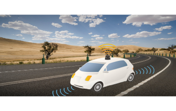
Let's suppose a self-driving car then PEAS representation will be:
Performance: Safety, time, legal drive, comfort
Environment: Roads, other vehicles, road signs, pedestrian
Actuators: Steering, accelerator, brake, signal, horn
Sensors: Camera, GPS, speedometer, odometer, accelerometer, sonar.
Example of Agents with their PEAS representation
Agent | Performance measure | Environment | Actuators | Sensors |
1. Medical Diagnose |
|
|
| Keyboard |
2. Vacuum Cleaner |
|
|
|
|
3. Part -picking Robot |
|
|
|
|
Problem-solving agents:
In Artificial Intelligence, Search techniques are universal problem-solving methods. Rational agents or Problem-solving agents in AI mostly used these search strategies or algorithms to solve a specific problem and provide the best result. Problem-solving agents are the goal-based agents and use atomic representation. In this topic, we will learn various problem-solving search algorithms.
Search Algorithm Terminologies:
- Search: Searchingis a step by step procedure to solve a search-problem in a given search space. A search problem can have three main factors:
- Search Space: Search space represents a set of possible solutions, which a system may have.
- Start State: It is a state from where agent begins the search.
- Goal test: It is a function which observe the current state and returns whether the goal state is achieved or not.
- Search tree: A tree representation of search problem is called Search tree. The root of the search tree is the root node which is corresponding to the initial state.
- Actions: It gives the description of all the available actions to the agent.
- Transition model: A description of what each action do, can be represented as a transition model.
- Path Cost: It is a function which assigns a numeric cost to each path.
- Solution: It is an action sequence which leads from the start node to the goal node.
- Optimal Solution: If a solution has the lowest cost among all solutions.
Properties of Search Algorithms:
Following are the four essential properties of search algorithms to compare the efficiency of these algorithms:
Completeness: A search algorithm is said to be complete if it guarantees to return a solution if at least any solution exists for any random input.
Optimality: If a solution found for an algorithm is guaranteed to be the best solution (lowest path cost) among all other solutions, then such a solution for is said to be an optimal solution.
Time Complexity: Time complexity is a measure of time for an algorithm to complete its task.
Space Complexity: It is the maximum storage space required at any point during the search, as the complexity of the problem.
Types of search algorithms
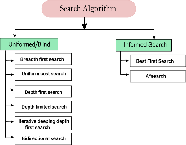
Based on the search problems we can classify the search algorithms into uninformed (Blind search) search and informed search (Heuristic search) algorithms.
Uninformed/Blind Search:
The uninformed search does not contain any domain knowledge such as closeness, the location of the goal. It operates in a brute-force way as it only includes information about how to traverse the tree and how to identify leaf and goal nodes. Uninformed search applies a way in which search tree is searched without any information about the search space like initial state operators and test for the goal, so it is also called blind search.It examines each node of the tree until it achieves the goal node.
It can be divided into five main types:
- Breadth-first search
- Uniform cost search
- Depth-first search
- Iterative deepening depth-first search
- Bidirectional Search
Informed Search
Informed search algorithms use domain knowledge. In an informed search, problem information is available which can guide the search. Informed search strategies can find a solution more efficiently than an uninformed search strategy. Informed search is also called a Heuristic search.
A heuristic is a way which might not always be guaranteed for best solutions but guaranteed to find a good solution in reasonable time.
Informed search can solve much complex problem which could not be solved in another way.
An example of informed search algorithms is a traveling salesman problem.
- Greedy Search
- A* Search
Uninformed Search Algorithms
Uninformed search is a class of general-purpose search algorithms which operates in brute force-way. Uninformed search algorithms do not have additional information about state or search space other than how to traverse the tree, so it is also called blind search.
Following are the various types of uninformed search algorithms:
- Breadth-first Search
- Depth-first Search
- Depth-limited Search
- Iterative deepening depth-first search
- Uniform cost search
- Bidirectional Search
1. Breadth-first Search:
- Breadth-first search is the most common search strategy for traversing a tree or graph. This algorithm searches breadthwise in a tree or graph, so it is called breadth-first search.
- BFS algorithm starts searching from the root node of the tree and expands all successor node at the current level before moving to nodes of next level.
- The breadth-first search algorithm is an example of a general-graph search algorithm.
- Breadth-first search implemented using FIFO queue data structure.
Advantages:
- BFS will provide a solution if any solution exists.
- If there are more than one solutions for a given problem, then BFS will provide the minimal solution which requires the least number of steps.
Disadvantages:
- It requires lots of memory since each level of the tree must be saved into memory to expand the next level.
- BFS needs lots of time if the solution is far away from the root node.
Example:
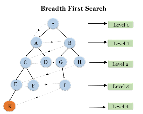
In the below tree structure, we have shown the traversing of the tree using BFS algorithm from the root node S to goal node K. BFS search algorithm traverse in layers, so it will follow the path which is shown by the dotted arrow, and the traversed path will be:
- S---> A--->B---->C--->D---->G--->H--->E---->F---->I---->K
Time Complexity: Time Complexity of BFS algorithm can be obtained by the number of nodes traversed in BFS until the shallowest Node. Where the d= depth of shallowest solution and b is a node at every state.
T (b) = 1+b2+b3+.......+ bd= O (bd)
Space Complexity: Space complexity of BFS algorithm is given by the Memory size of frontier which is O(bd).
Completeness: BFS is complete, which means if the shallowest goal node is at some finite depth, then BFS will find a solution.
Optimality: BFS is optimal if path cost is a non-decreasing function of the depth of the node.
2. Depth-first Search
- Depth-first search isa recursive algorithm for traversing a tree or graph data structure.
- It is called the depth-first search because it starts from the root node and follows each path to its greatest depth node before moving to the next path.
- DFS uses a stack data structure for its implementation.
- The process of the DFS algorithm is similar to the BFS algorithm.
Note: Backtracking is an algorithm technique for finding all possible solutions using recursion.
Advantage:
- DFS requires very less memory as it only needs to store a stack of the nodes on the path from root node to the current node.
- It takes less time to reach to the goal node than BFS algorithm (if it traverses in the right path).
Disadvantage:
- There is the possibility that many states keep re-occurring, and there is no guarantee of finding the solution.
- DFS algorithm goes for deep down searching and sometime it may go to the infinite loop.
Example:
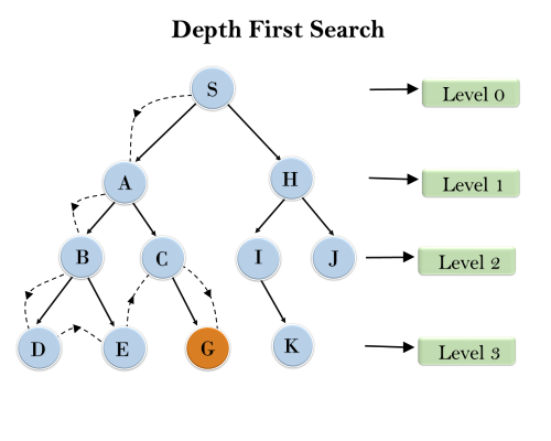
In the below search tree, we have shown the flow of depth-first search, and it will follow the order as:
Root node--->Left node ----> right node.
It will start searching from root node S, and traverse A, then B, then D and E, after traversing E, it will backtrack the tree as E has no other successor and still goal node is not found. After backtracking it will traverse node C and then G, and here it will terminate as it found goal node.
Completeness: DFS search algorithm is complete within finite state space as it will expand every node within a limited search tree.
Time Complexity: Time complexity of DFS will be equivalent to the node traversed by the algorithm. It is given by:
T(n)= 1+ n2+ n3 +.........+ nm=O(nm)
Where, m= maximum depth of any node and this can be much larger than d (Shallowest solution depth)
Space Complexity: DFS algorithm needs to store only single path from the root node, hence space complexity of DFS is equivalent to the size of the fringe set, which is O(bm).
Optimal: DFS search algorithm is non-optimal, as it may generate a large number of steps or high cost to reach to the goal node.
3. Depth-Limited Search Algorithm:
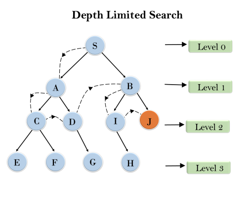
A depth-limited search algorithm is similar to depth-first search with a predetermined limit. Depth-limited search can solve the drawback of the infinite path in the Depth-first search. In this algorithm, the node at the depth limit will treat as it has no successor nodes further.
Depth-limited search can be terminated with two Conditions of failure:
- Standard failure value: It indicates that problem does not have any solution.
- Cutoff failure value: It defines no solution for the problem within a given depth limit.
Advantages:
Depth-limited search is Memory efficient.
Disadvantages:
- Depth-limited search also has a disadvantage of incompleteness.
- It may not be optimal if the problem has more than one solution.
Example:
Completeness: DLS search algorithm is complete if the solution is above the depth-limit.
Time Complexity: Time complexity of DLS algorithm is O(bℓ).
Space Complexity: Space complexity of DLS algorithm is O(b×ℓ).
Optimal: Depth-limited search can be viewed as a special case of DFS, and it is also not optimal even if ℓ>d.
4. Uniform-cost Search Algorithm:
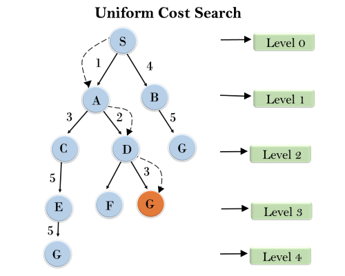
Uniform-cost search is a searching algorithm used for traversing a weighted tree or graph. This algorithm comes into play when a different cost is available for each edge. The primary goal of the uniform-cost search is to find a path to the goal node which has the lowest cumulative cost. Uniform-cost search expands nodes according to their path costs form the root node. It can be used to solve any graph/tree where the optimal cost is in demand. A uniform-cost search algorithm is implemented by the priority queue. It gives maximum priority to the lowest cumulative cost. Uniform cost search is equivalent to BFS algorithm if the path cost of all edges is the same.
Advantages:
- Uniform cost search is optimal because at every state the path with the least cost is chosen.
Disadvantages:
- It does not care about the number of steps involve in searching and only concerned about path cost. Due to which this algorithm may be stuck in an infinite loop.
Example:
Completeness:
Uniform-cost search is complete, such as if there is a solution, UCS will find it.
Time Complexity:
Let C* is Cost of the optimal solution, and ε is each step to get closer to the goal node. Then the number of steps is = C*/ε+1. Here we have taken +1, as we start from state 0 and end to C*/ε.
Hence, the worst-case time complexity of Uniform-cost search isO(b1 + [C*/ε])/.
Space Complexity:
The same logic is for space complexity so, the worst-case space complexity of Uniform-cost search is O(b1 + [C*/ε]).
Optimal:
Uniform-cost search is always optimal as it only selects a path with the lowest path cost.
5. Iterative deepeningdepth-first Search:
The iterative deepening algorithm is a combination of DFS and BFS algorithms. This search algorithm finds out the best depth limit and does it by gradually increasing the limit until a goal is found.
This algorithm performs depth-first search up to a certain "depth limit", and it keeps increasing the depth limit after each iteration until the goal node is found.
This Search algorithm combines the benefits of Breadth-first search's fast search and depth-first search's memory efficiency.
The iterative search algorithm is useful uninformed search when search space is large, and depth of goal node is unknown.
Advantages:
- Itcombines the benefits of BFS and DFS search algorithm in terms of fast search and memory efficiency.
Disadvantages:
- The main drawback of IDDFS is that it repeats all the work of the previous phase.
Example:
Following tree structure is showing the iterative deepening depth-first search. IDDFS algorithm performs various iterations until it does not find the goal node. The iteration performed by the algorithm is given as:
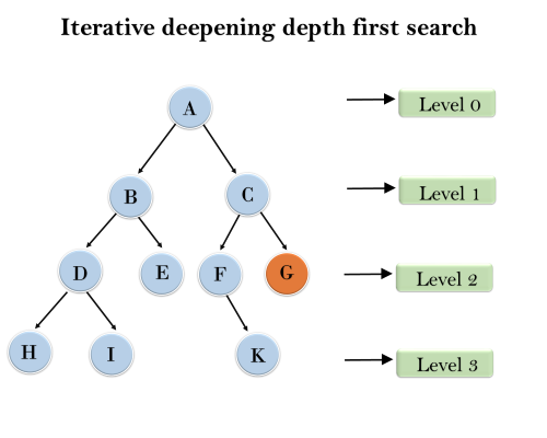
1'st Iteration-----> A
2'nd Iteration----> A, B, C
3'rd Iteration------>A, B, D, E, C, F, G
4'th Iteration------>A, B, D, H, I, E, C, F, K, G
In the fourth iteration, the algorithm will find the goal node.
Completeness:
This algorithm is complete is ifthe branching factor is finite.
Time Complexity:
Let's suppose b is the branching factor and depth is d then the worst-case time complexity is O(bd).
Space Complexity:
The space complexity of IDDFS will be O(bd).
Optimal:
IDDFS algorithm is optimal if path cost is a non- decreasing function of the depth of the node.
6. Bidirectional Search Algorithm:
Bidirectional search algorithm runs two simultaneous searches, one form initial state called as forward-search and other from goal node called as backward-search, to find the goal node. Bidirectional search replaces one single search graph with two small subgraphs in which one starts the search from an initial vertex and other starts from goal vertex. The search stops when these two graphs intersect each other.
Bidirectional search can use search techniques such as BFS, DFS, DLS, etc.
Advantages:
- Bidirectional search is fast.
- Bidirectional search requires less memory
Disadvantages:
- Implementation of the bidirectional search tree is difficult.
- In bidirectional search, one should know the goal state in advance.
Example:
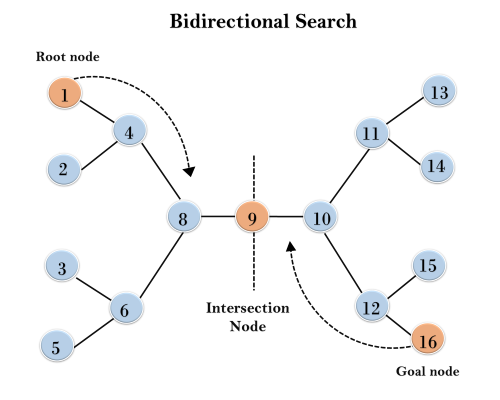
In the below search tree, bidirectional search algorithm is applied. This algorithm divides one graph/tree into two sub-graphs. It starts traversing from node 1 in the forward direction and starts from goal node 16 in the backward direction.
The algorithm terminates at node 9 where two searches meet.
Completeness: Bidirectional Search is complete if we use BFS in both searches.
Time Complexity: Time complexity of bidirectional search using BFS is O(bd).
Space Complexity: Space complexity of bidirectional search is O(bd).
Optimal: Bidirectional search is Optimal.
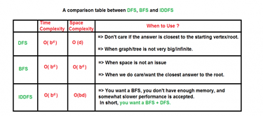
There are two common ways to traverse a graph, BFS and DFS. Considering a Tree (or Graph) of huge height and width, both BFS and DFS are not very efficient due to following reasons.
- DFS first traverses nodes going through one adjacent of root, then next adjacent. The problem with this approach is, if there is a node close to root, but not in first few subtrees explored by DFS, then DFS reaches that node very late. Also, DFS may not find shortest path to a node (in terms of number of edges).
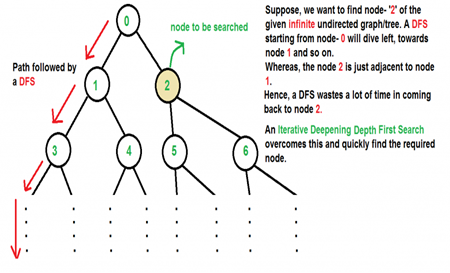
2. BFS goes level by level, but requires more space. The space required by DFS is O(d) where d is depth of tree, but space required by BFS is O(n) where n is number of nodes in tree (Why? Note that the last level of tree can have around n/2 nodes and second last level n/4 nodes and in BFS we need to have every level one by one in queue).
IDDFS combines depth-first search’s space-efficiency and breadth-first search’s fast search (for nodes closer to root).
How does IDDFS work?
IDDFS calls DFS for different depths starting from an initial value. In every call, DFS is restricted from going beyond given depth. So basically we do DFS in a BFS fashion.
Algorithm:
// Returns true if target is reachable from
// src within max_depth
Bool IDDFS(src, target, max_depth)
For limit from 0 to max_depth
If DLS(src, target, limit) == true
Return true
Return false
Bool DLS(src, target, limit)
If (src == target)
Return true;
// If reached the maximum depth,
// stop recursing.
If (limit <= 0)
Return false;
Foreach adjacent i of src
If DLS(i, target, limit?1)
Return true
Return false
An important thing to note is, we visit top level nodes multiple times. The last (or max depth) level is visited once, second last level is visited twice, and so on. It may seem expensive, but it turns out to be not so costly, since in a tree most of the nodes are in the bottom level. So it does not matter much if the upper levels are visited multiple times.
Below is implementation of above algorithm
// C++ program to search if a target node is reachable from // a source with given max depth. #include<bits/stdc++.h> Using namespace std;
// Graph class represents a directed graph using adjacency // list representation. Class Graph { Int V; // No. Of vertices
// Pointer to an array containing // adjacency lists List<int> *adj;
// A function used by IDDFS Bool DLS(int v, int target, int limit);
Public: Graph(int V); // Constructor Void addEdge(int v, int w);
// IDDFS traversal of the vertices reachable from v Bool IDDFS(int v, int target, int max_depth); };
Graph::Graph(int V) { This->V = V; Adj = new list<int>[V]; }
Void Graph::addEdge(int v, int w) { Adj[v].push_back(w); // Add w to v’s list. }
// A function to perform a Depth-Limited search // from given source 'src' Bool Graph::DLS(int src, int target, int limit) { If (src == target) Return true;
// If reached the maximum depth, stop recursing. If (limit <= 0) Return false;
// Recur for all the vertices adjacent to source vertex For (auto i = adj[src].begin(); i != adj[src].end(); ++i) If (DLS(*i, target, limit-1) == true) Return true;
Return false; }
// IDDFS to search if target is reachable from v. // It uses recursive DFSUtil(). Bool Graph::IDDFS(int src, int target, int max_depth) { // Repeatedly depth-limit search till the // maximum depth. For (int i = 0; i <= max_depth; i++) If (DLS(src, target, i) == true) Return true;
Return false; }
// Driver code Int main() { // Let us create a Directed graph with 7 nodes Graph g(7); g.addEdge(0, 1); g.addEdge(0, 2); g.addEdge(1, 3); g.addEdge(1, 4); g.addEdge(2, 5); g.addEdge(2, 6);
Int target = 6, maxDepth = 3, src = 0; If (g.IDDFS(src, target, maxDepth) == true) Cout << "Target is reachable from source " "within max depth"; Else Cout << "Target is NOT reachable from source " "within max depth"; Return 0; } |
Output :
Target is reachable from source within max depth
Illustration:
There can be two cases-
a) When the graph has no cycle: This case is simple. We can DFS multiple times with different height limits.
b) When the graph has cycles. This is interesting as there is no visited flag in IDDFS.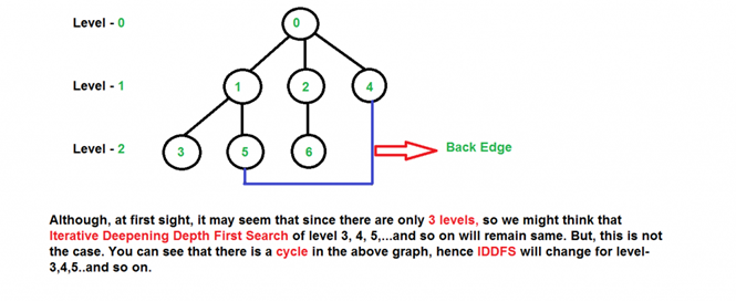
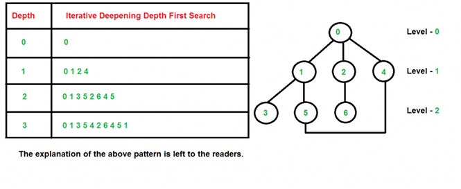
Time Complexity: Suppose we have a tree having branching factor ‘b’ (number of children of each node), and its depth ‘d’, i.e., there are bd nodes.
In an iterative deepening search, the nodes on the bottom level are expanded once, those on the next to bottom level are expanded twice, and so on, up to the root of the search tree, which is expanded d+1 times. So the total number of expansions in an iterative deepening search is-
(d)b + (d-1)b2 + .... + 3bd-2 + 2bd-1 + bd
That is,
Summation[(d + 1 - i) bi], from i = 0 to i = d
Which is same as O(bd)
After evaluating the above expression, we find that asymptotically IDDFS takes the same time as that of DFS and BFS, but it is indeed slower than both of them as it has a higher constant factor in its time complexity expression.
IDDFS is best suited for a complete infinite tree
Heuristics function: Heuristic is a function which is used in Informed Search, and it finds the most promising path. It takes the current state of the agent as its input and produces the estimation of how close agent is from the goal. The heuristic method, however, might not always give the best solution, but it guaranteed to find a good solution in reasonable time. Heuristic function estimates how close a state is to the goal. It is represented by h(n), and it calculates the cost of an optimal path between the pair of states. The value of the heuristic function is always positive.
Admissibility of the heuristic function is given as:
- h(n) <= h*(n)
Here h(n) is heuristic cost, and h*(n) is the estimated cost. Hence heuristic cost should be less than or equal to the estimated cost.
Pure Heuristic Search:
Pure heuristic search is the simplest form of heuristic search algorithms. It expands nodes based on their heuristic value h(n). It maintains two lists, OPEN and CLOSED list. In the CLOSED list, it places those nodes which have already expanded and in the OPEN list, it places nodes which have yet not been expanded.
On each iteration, each node n with the lowest heuristic value is expanded and generates all its successors and n is placed to the closed list. The algorithm continues unit a goal state is found.
In the informed search we will discuss two main algorithms which are given below:
- Best First Search Algorithm(Greedy search)
- A* Search Algorithm
Any finite CSP can be solved by an exhaustive generate-and-test algorithm. The assignment space, D, is the set of assignments of values to all of the variables; it corresponds to the set of all possible worlds. Each element of D is a total assignment of a value to each variable. The algorithm returns those assignments that satisfy all of the constraints.
Thus, the generate-and-test algorithm is as follows: check each total assignment in turn; if an assignment is found that satisfies all of the constraints, return that assignment.
Example 4.11:
D | ={ | {A=1,B=1,C=1,D=1,E=1}, |
|
| {A=1,B=1,C=1,D=1,E=2},..., |
|
| {A=4,B=4,C=4,D=4,E=4}}. |
In this case there are |D|=45=1,024 different assignments to be tested. In the crossword there are 406=4,096,000,000 possible assignments.
If each of the n variable domains has size d, then D has dn elements. If there are e constraints, the total number of constraints tested is O(edn). As n becomes large, this very quickly becomes intractable, and so we must find alternative solution methods.
Best-first Search Algorithm (Greedy Search):
Greedy best-first search algorithm always selects the path which appears best at that moment. It is the combination of depth-first search and breadth-first search algorithms. It uses the heuristic function and search. Best-first search allows us to take the advantages of both algorithms. With the help of best-first search, at each step, we can choose the most promising node. In the best first search algorithm, we expand the node which is closest to the goal node and the closest cost is estimated by heuristic function, i.e.
- f(n)= g(n).
Were, h(n)= estimated cost from node n to the goal.
The greedy best first algorithm is implemented by the priority queue.
Best first search algorithm:
- Step 1: Place the starting node into the OPEN list.
- Step 2: If the OPEN list is empty, Stop and return failure.
- Step 3: Remove the node n, from the OPEN list which has the lowest value of h(n), and places it in the CLOSED list.
- Step 4: Expand the node n, and generate the successors of node n.
- Step 5: Check each successor of node n, and find whether any node is a goal node or not. If any successor node is goal node, then return success and terminate the search, else proceed to Step 6.
- Step 6: For each successor node, algorithm checks for evaluation function f(n), and then check if the node has been in either OPEN or CLOSED list. If the node has not been in both list, then add it to the OPEN list.
- Step 7: Return to Step 2.
Advantages:
- Best first search can switch between BFS and DFS by gaining the advantages of both the algorithms.
- This algorithm is more efficient than BFS and DFS algorithms.
Disadvantages:
- It can behave as an unguided depth-first search in the worst case scenario.
- It can get stuck in a loop as DFS.
- This algorithm is not optimal.
Example:
Consider the below search problem, and we will traverse it using greedy best-first search. At each iteration, each node is expanded using evaluation function f(n)=h(n) , which is given in the below table.
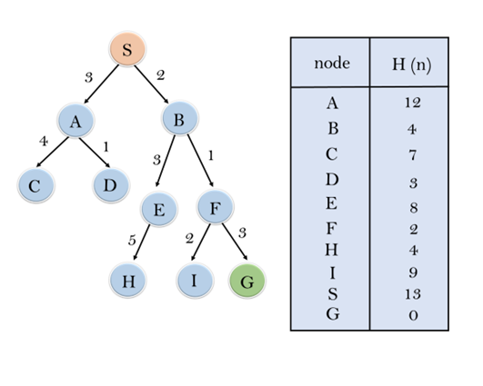
In this search example, we are using two lists which are OPEN and CLOSED Lists. Following are the iteration for traversing the above example.
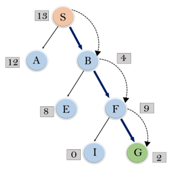
Expand the nodes of S and put in the CLOSED list
Initialization: Open [A, B], Closed [S]
Iteration 1: Open [A], Closed [S, B]
Iteration 2: Open [E, F, A], Closed [S, B]
: Open [E, A], Closed [S, B, F]
Iteration 3: Open [I, G, E, A], Closed [S, B, F]
: Open [I, E, A], Closed [S, B, F, G]
Hence the final solution path will be: S----> B----->F----> G
Time Complexity: The worst case time complexity of Greedy best first search is O(bm).
Space Complexity: The worst case space complexity of Greedy best first search is O(bm). Where, m is the maximum depth of the search space.
Complete: Greedy best-first search is also incomplete, even if the given state space is finite.
Optimal: Greedy best first search algorithm is not optimal.
What is Beam search?
To understand the Beam search, we will use the neural machine translation use case of sequence of sequence.
The sequence to sequence model uses an encoder and decoder framework with Long Short Term Memory(LSTM) or Gated Recurrent Unit(GRU) as the basic blocks.
Encoder maps a source sequence encodes the source information and passes it to the decoder. The decoder takes the encoded data from the encoder as an input along with the start-of-string <START> token as the initial input to produce an output sequence.
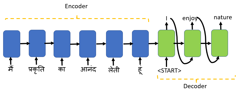
Here the source sequence is a sentence in Hindi, and the target sequence is generated in English. You don’t want any random English translation, but you would like the best and most likely words to be selected for the translation that matches the meaning of the Hindi sentence.
I have examples in Hindi as that is the other language other than English that I know.
How do you select the best and most likely words for the target sequence?
A simple approach would be to have a vocabulary of words in the target language, say 10,000 words then, based on the source sentence, get a probability for each of the 10,000 target words.
There could be multiple likely translations of the source sentence in the target language.
Should you pick any translation randomly?
Our goal is to pick the best and most likely translated word, so we choose the target word with the maximum probability based on the source sentence.
Should you pick only one best translation?
Greedy Search algorithm selects one best candidate as an input sequence for each time step. Choosing just one best candidate might be suitable for the current time step, but when we construct the full sentence, it may be a sub-optimal choice.
The beam search algorithm selects multiple alternatives for an input sequence at each timestep based on conditional probability. The number of multiple alternatives depends on a parameter called Beam Width B. At each time step, the beam search selects B number of best alternatives with the highest probability as the most likely possible choices for the time step.
Let’s take an example to understand this.

We will select the beam width =3; our vocabulary of English words is 10,000.
Step 1:Find the top 3 words with the highest probability given the input sentence. The number of most likely words are based on the beam width
- Input the encoded input sentence to the decoder; the decoder will then apply softmax function to all the 10,000 words in the vocabulary.
- From 10,000 possibilities, we will select only the top 3 words with the highest probability.
- Consider three best and most likely alternative for the translated word as the beam width is set to three.
- If the beam width is set 10, then we will select the top 10 words with the highest probability. We store the top 3 words: I, My and We in the memory
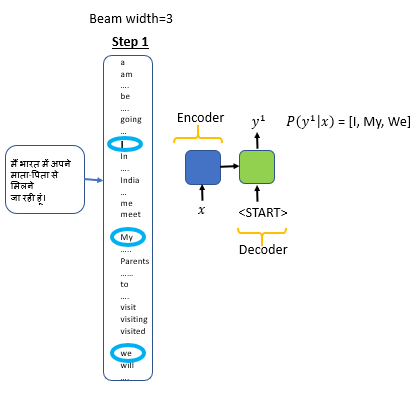
Step 1:Find three words with the highest probability based on the input sentence
Greedy Search will always consider only one best alternative.
Step 2: Find the three best pairs for the first and second words based on conditional probability
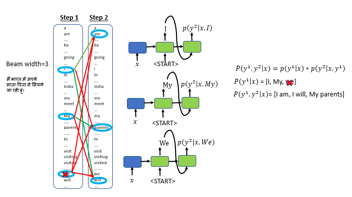
Step 2: Find the top 3 pair of words for the first and second word of the translated sentence
- Take the first three selected words(I, My, We) from step1 as input to the second step
- Apply the softmax function to all the 10,000 words in the vocabulary to find the three best alternatives for the second word. While doing this, we will figure out the combination of the first and second words that are most likely to form a pair using conditional probability.
- To find the three best pairs for the first and second words, we will take the first word “I”, apply the softmax function to all the 10,000 words in the vocabulary.
- Evaluate the probability for the other two words select first words: “My: and “We”
- Run 30,000 different combinations to choose the top 3 pairs of the first and the second words.
- The top 3 first and second-word pair combinations are: “I am”, “My parents”, and “I will”
- We have now dropped the first word “We” as we did not find any word pair with “We” as the first and second word having a high conditional probability
- At every step, we instantiate three copies of the encoder-decoder network to evaluate these partial sentence fragments and the output. Number of copies of the network is the same as the size of the beam width
Step 3: Find the three best pairs for the first, second and third word based on the input sentence and the chosen first and the second word
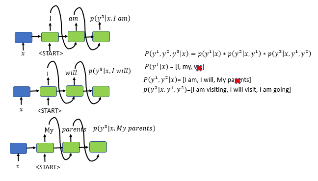
Step 3: find the most likely choice of the first three words in the translated sentence
- Along with the input sentence and the top 3 first and second-word pair combinations: “I am”, “My parents”, and “I will”, find the third word with the highest conditional probability.
- Again run 30,000 combinations to select the best and most likely combination of the first, the second and the third word and instantiate three copies of the seq2seq, encoder-decoder model
- The top 3 first, second, and third-word combinations are: “I am visiting”, “I will visit”, and “l am going”.
- We drop the combination “My parents” as we did not find the first, second, and third-word combinations with “My parents” within the top 3 combinations.
We continue this process, and we pick three sentences with the highest probability. The top 3 sentences can vary in length or maybe the same length.

Three output sentences with the highest conditional probabilities and different lengths
We finally pick the output of the decoder as the sentence with the highest probability

Will a higher value for the beam width give a better translation?
A higher beam width will give a better translation but would use a lot of memory and computational power.
When we had a beamwidth of 3 and 10,000-word vocabulary, we evaluated 30,000 combinations at each time step, created three instances of the encoder-decoder, and max sentence length was 9. Creating multiple copies of encoder-decoder and calculating conditional probabilities for 30,000 words at each time step needs lots of memory and computation power.
A lower beam width will result in more inferior quality translation but will be fast and efficient in terms of memory usage and computational power
Hill Climbing Algorithm in Artificial Intelligence
- Hill climbing algorithm is a local search algorithm which continuously moves in the direction of increasing elevation/value to find the peak of the mountain or best solution to the problem. It terminates when it reaches a peak value where no neighbor has a higher value.
- Hill climbing algorithm is a technique which is used for optimizing the mathematical problems. One of the widely discussed examples of Hill climbing algorithm is Traveling-salesman Problem in which we need to minimize the distance traveled by the salesman.
- It is also called greedy local search as it only looks to its good immediate neighbor state and not beyond that.
- A node of hill climbing algorithm has two components which are state and value.
- Hill Climbing is mostly used when a good heuristic is available.
- In this algorithm, we don't need to maintain and handle the search tree or graph as it only keeps a single current state.
Features of Hill Climbing:
Following are some main features of Hill Climbing Algorithm:
- Generate and Test variant: Hill Climbing is the variant of Generate and Test method. The Generate and Test method produce feedback which helps to decide which direction to move in the search space.
- Greedy approach: Hill-climbing algorithm search moves in the direction which optimizes the cost.
- No backtracking: It does not backtrack the search space, as it does not remember the previous states.
State-space Diagram for Hill Climbing:
The state-space landscape is a graphical representation of the hill-climbing algorithm which is showing a graph between various states of algorithm and Objective function/Cost.
On Y-axis we have taken the function which can be an objective function or cost function, and state-space on the x-axis. If the function on Y-axis is cost then, the goal of search is to find the global minimum and local minimum. If the function of Y-axis is Objective function, then the goal of the search is to find the global maximum and local maximum.
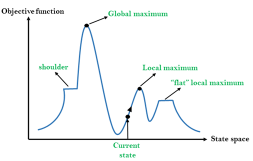
Different regions in the state space landscape:
Local Maximum: Local maximum is a state which is better than its neighbor states, but there is also another state which is higher than it.
Global Maximum: Global maximum is the best possible state of state space landscape. It has the highest value of objective function.
Current state: It is a state in a landscape diagram where an agent is currently present.
Flat local maximum: It is a flat space in the landscape where all the neighbor states of current states have the same value.
Shoulder: It is a plateau region which has an uphill edge.
Types of Hill Climbing Algorithm:
- Simple hill Climbing:
- Steepest-Ascent hill-climbing:
- Stochastic hill Climbing:
1. Simple Hill Climbing:
Simple hill climbing is the simplest way to implement a hill climbing algorithm. It only evaluates the neighbor node state at a time and selects the first one which optimizes current cost and set it as a current state. It only checks it's one successor state, and if it finds better than the current state, then move else be in the same state. This algorithm has the following features:
- Less time consuming
- Less optimal solution and the solution is not guaranteed
Algorithm for Simple Hill Climbing:
- Step 1: Evaluate the initial state, if it is goal state then return success and Stop.
- Step 2: Loop Until a solution is found or there is no new operator left to apply.
- Step 3: Select and apply an operator to the current state.
- Step 4: Check new state:
- If it is goal state, then return success and quit.
- Else if it is better than the current state then assign new state as a current state.
- Else if not better than the current state, then return to step2.
- Step 5: Exit.
2. Steepest-Ascent hill climbing:
The steepest-Ascent algorithm is a variation of simple hill climbing algorithm. This algorithm examines all the neighboring nodes of the current state and selects one neighbor node which is closest to the goal state. This algorithm consumes more time as it searches for multiple neighbors
Algorithm for Steepest-Ascent hill climbing:
- Step 1: Evaluate the initial state, if it is goal state then return success and stop, else make current state as initial state.
- Step 2: Loop until a solution is found or the current state does not change.
- Let SUCC be a state such that any successor of the current state will be better than it.
- For each operator that applies to the current state:
- Apply the new operator and generate a new state.
- Evaluate the new state.
- If it is goal state, then return it and quit, else compare it to the SUCC.
- If it is better than SUCC, then set new state as SUCC.
- If the SUCC is better than the current state, then set current state to SUCC.
- Step 5: Exit.
3. Stochastic hill climbing:
Stochastic hill climbing does not examine for all its neighbor before moving. Rather, this search algorithm selects one neighbor node at random and decides whether to choose it as a current state or examine another state.
Problems in Hill Climbing Algorithm:
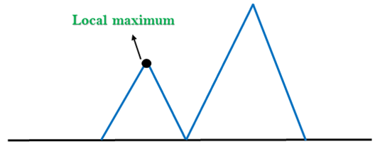
1. Local Maximum: A local maximum is a peak state in the landscape which is better than each of its neighboring states, but there is another state also present which is higher than the local maximum.
Solution: Backtracking technique can be a solution of the local maximum in state space landscape. Create a list of the promising path so that the algorithm can backtrack the search space and explore other paths as well.
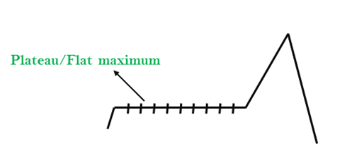
2. Plateau: A plateau is the flat area of the search space in which all the neighbor states of the current state contains the same value, because of this algorithm does not find any best direction to move. A hill-climbing search might be lost in the plateau area.
Solution: The solution for the plateau is to take big steps or very little steps while searching, to solve the problem. Randomly select a state which is far away from the current state so it is possible that the algorithm could find non-plateau region.
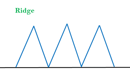
3. Ridges: A ridge is a special form of the local maximum. It has an area which is higher than its surrounding areas, but itself has a slope, and cannot be reached in a single move.
Solution: With the use of bidirectional search, or by moving in different directions, we can improve this problem.
Simulated Annealing:
A hill-climbing algorithm which never makes a move towards a lower value guaranteed to be incomplete because it can get stuck on a local maximum. And if algorithm applies a random walk, by moving a successor, then it may complete but not efficient. Simulated Annealing is an algorithm which yields both efficiency and completeness.
In mechanical term Annealing is a process of hardening a metal or glass to a high temperature then cooling gradually, so this allows the metal to reach a low-energy crystalline state. The same process is used in simulated annealing in which the algorithm picks a random move, instead of picking the best move. If the random move improves the state, then it follows the same path. Otherwise, the algorithm follows the path which has a probability of less than 1 or it moves downhill and chooses another path.
A* search is the most commonly known form of best-first search. It uses heuristic function h(n), and cost to reach the node n from the start state g(n). It has combined features of UCS and greedy best-first search, by which it solve the problem efficiently. A* search algorithm finds the shortest path through the search space using the heuristic function. This search algorithm expands less search tree and provides optimal result faster. A* algorithm is similar to UCS except that it uses g(n)+h(n) instead of g(n).
In A* search algorithm, we use search heuristic as well as the cost to reach the node. Hence we can combine both costs as following, and this sum is called as a fitness number.

At each point in the search space, only those node is expanded which have the lowest value of f(n), and the algorithm terminates when the goal node is found.
Algorithm of A* search:
Step1: Place the starting node in the OPEN list.
Step 2: Check if the OPEN list is empty or not, if the list is empty then return failure and stops.
Step 3: Select the node from the OPEN list which has the smallest value of evaluation function (g+h), if node n is goal node then return success and stop, otherwise
Step 4: Expand node n and generate all of its successors, and put n into the closed list. For each successor n', check whether n' is already in the OPEN or CLOSED list, if not then compute evaluation function for n' and place into Open list.
Step 5: Else if node n' is already in OPEN and CLOSED, then it should be attached to the back pointer which reflects the lowest g(n') value.
Step 6: Return to Step 2.
Advantages:
- A* search algorithm is the best algorithm than other search algorithms.
- A* search algorithm is optimal and complete.
- This algorithm can solve very complex problems.
Disadvantages:
- It does not always produce the shortest path as it mostly based on heuristics and approximation.
- A* search algorithm has some complexity issues.
- The main drawback of A* is memory requirement as it keeps all generated nodes in the memory, so it is not practical for various large-scale problems.
Example:
In this example, we will traverse the given graph using the A* algorithm. The heuristic value of all states is given in the below table so we will calculate the f(n) of each state using the formula f(n)= g(n) + h(n), where g(n) is the cost to reach any node from start state.
Here we will use OPEN and CLOSED list.
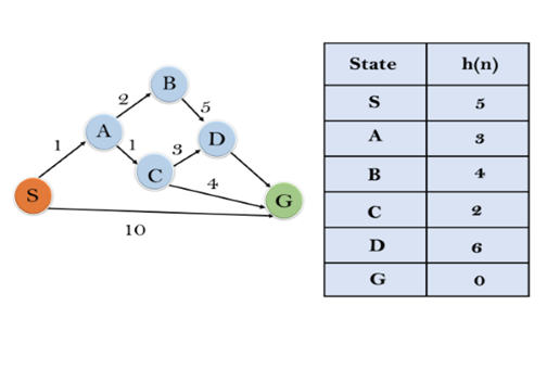
Solution:
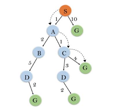
Initialization: {(S, 5)}
Iteration1: {(S--> A, 4), (S-->G, 10)}
Iteration2: {(S--> A-->C, 4), (S--> A-->B, 7), (S-->G, 10)}
Iteration3: {(S--> A-->C--->G, 6), (S--> A-->C--->D, 11), (S--> A-->B, 7), (S-->G, 10)}
Iteration 4 will give the final result, as S--->A--->C--->G it provides the optimal path with cost 6.
Points to remember:
- A* algorithm returns the path which occurred first, and it does not search for all remaining paths.
- The efficiency of A* algorithm depends on the quality of heuristic.
- A* algorithm expands all nodes which satisfy the condition f(n) <="" li="">
Complete: A* algorithm is complete as long as:
- Branching factor is finite.
- Cost at every action is fixed.
Optimal: A* search algorithm is optimal if it follows below two conditions:
- Admissible: the first condition requires for optimality is that h(n) should be an admissible heuristic for A* tree search. An admissible heuristic is optimistic in nature.
- Consistency: Second required condition is consistency for only A* graph-search.
If the heuristic function is admissible, then A* tree search will always find the least cost path.
Time Complexity: The time complexity of A* search algorithm depends on heuristic function, and the number of nodes expanded is exponential to the depth of solution d. So the time complexity is O(b^d), where b is the branching factor.
Space Complexity: The space complexity of A* search algorithm is O(b^d)
Search
- a tool for problem solving of AI applications.
- Typical problem includes:
- Finding the solution to a puzzle e.g. The 8-puzzle
- Finding a proof for a theorem in logic or mathematics
- Finding the shortest path connecting a set of non-equidistant points (the TSP traveling salesman problem)
- Finding a sequence of moves that will win a game, or the best move to make at a given point in a game.
[Note that one cannot explore all possible moves until end games, unless the game is simple, such as tic-tac-toe.] - Finding a sequence of transformations that will solve a symbolic integration problem.
- Problem Representation
- State space representation
- Problem reduction representation
- Game tree
- Search method
- Blind state-space search
- Blind AND/OR graph search
- Heuristic state-space search (A*)
- Heuristic search of an AND/OR graph
- Game tree search
Components of Search Systems
- Problem solving systems can be described in terms of 3 main components:
- A Database
- Describes both the current task domain situation and the goal
- Consists of variety of different kinds of data structures
e.g. Arrays, lists, sets of predicates calculus expressions, property lists, semantic networks, ... - In Chess playing:
- Current situation - chess board configurations
- Goal - a winning board configuration
- In theorem proving:
- Current situation - assertions representing axioms, lemmas and theorem already proved.
- Goal - assertion representing the theorem to be proved.
- In information retrieval application
- Current situation - a set of facts
- Goal - query to be answered
- In robot problem solving
- Current situation - a world model consisting of statements describing the physical surroundings of the robot
- Goal - a description that is to be made true by a sequence of robot actions
2. A Set of Operators
- Used to manipulate the database
- In chess, rules for moving chessman
- In theorem proving, rules of inference such as modus ponens and resolution.
- In symbolic integration, rules for simplifying the form to be integrated (e.g. Integration by parts)
3. A Control Strategy
- Decide what to do next
e.g. What operator to apply and where to apply
Note that the choice of control strategy affects the contents and organization of the database.
The objectives: to achieve the goal by applying an appropriate sequence of operators to an initial task domain situation.
- Each application of the operator modifies the situation
- Representation will maintain data structures showing the effects of each alternative sequence.
- Control strategy investigate (search) various operator sequences in parallel that looks "promising".
[If description of task domain is too large, multiple version cannot be stored, and backtracking may be required.]
Reasoning forward & backward
Reasoning forward
- Application of operators to produce a modified situation, forward from its initial configuration to one satisfying a goal situation.
- For example, robot will start from current location and explore forwards.
- Said to be data driven or bottom-up. (The goal is at the top)
Reasoning backward

- The goal statement is converted to one or more sub-goals that are (hopefully) easier to solve and whose solutions are sufficient to solve the original problem, e.g.
- Said to be goal-directed or top-down.
- Much human problem-solving behaviour is observed to involve reasoning backwards. (Many AI programs are based on this strategy).
- Can combine forward and backward reasoning.
Graph Representation
- Tree structure is commonly used. The nodes (states) are connected together. The descendent of a node is the nodes (states) that can be reached from the current node.
- In general, graph structure is needed, because you may have repeated states.
- For problem reduction, a node can be solved only if ALL of its sub-problem can be solved. (e.g. Integration by parts will require all parts to be integrated.).
- Use AND/OR graph.
- Game Tree representation for game playing involving two opponents. Each player will try to maximize his own advantage.
- Many problem have infinite search space, or unimaginably large search space (e.g. Chess, go etc), and cannot search the entire space. Must stop and do an estimation on the goodness of the node at some time.
- Need to expand the node when required, cannot store the entire search space.
- Have to limit the search - exhaustive search is rarely feasible in non-trivial problems (combinatorial explosion)
- Use of heuristic knowledge from the problem domain to help focus the search.
State spaces Representation of Problems
- State spaces are spaces of states [!]
- Each situation (or configurations) is represented by a state, usually in the form of node of a graph.
- There is an initial state and final state representing the initial and final configuration. (e.g. In chess playing, the initial state is just the startup board configuration, while the final state is any winning configuration)
- Arcs exists from node A to node B if you can move within 1 step from configuration A to configuration B.
- Objective: to find a path from the initial state to a final state, usually via searching.
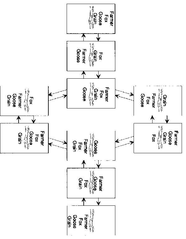
- Example: (farmer, fox, goose and grain)
A farmer wants to move himself, a silver fox, a fat goose and some tasty grain across a river. Unfortunately, his goat is so tiny he can take only one of his possessions across on any trip. Worse yet, an unattended fox will eat a goose, and an unattended goose will eat grain, so the farmer must not leave the fox alone with the goose or the goose alone with the grain. What is he to do? - Each state can be represented by a 4-tuple, e.g. [L R L R], representing the location of framer, fox, goose and grain respectively. L 0 left side of river, R 0 right side of river.
- Initial state: [L L L L], final state: [R R R R]
- Some state are not allowed by problem description, e.g. [L L R R], where the goose and grain are on the same side of the river.
- Also, not all nodes are connected by arcs, because the boat must be operated by the farmer, and the above rule also applies on the boat.
Example: (8-puzzle)
2 | 1 | 6 |
4 |
| 8 |
7 | 5 | 3 |
Initial Configuration
1 | 2 | 3 |
8 |
| 4 |
7 | 6 | 5 |
Solution Configuration
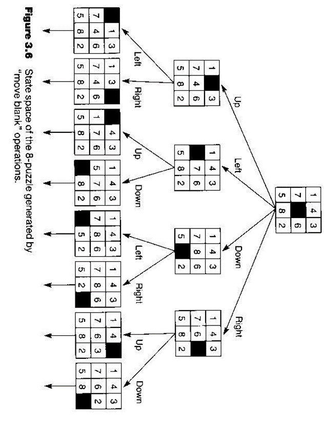
A tile may be moved by sliding it vertically or horizontally into an empty square.
State: represented by a 3x3 matrix as above.
Operators: instead of sliding the tile, represented as moving the empty square: UP, DOWN, LEFT, RIGHT.
There are a total of 181,440 possible states.
a common variation of state-space problem require finding not just any path but one of minimum cost between an initial node and a goal node. e.g. Traveling Salesman Problem
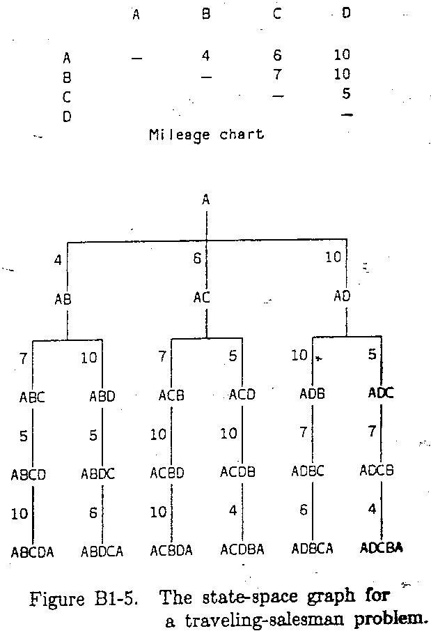
Sometimes the state-space graph is too large to be represented explicitly. The problem becomes generating just enough of the graph to contain the desired solution paths.
Problem Reduction Representation
Consists of 3 parts
Initail problem description
a set of operators for transforming problems to sub-problems
a set of primitive descriptions (whose solution is immediate)
Reasoning proceeds backwards from the initial goal.
Example: (Tower of Hanoi)
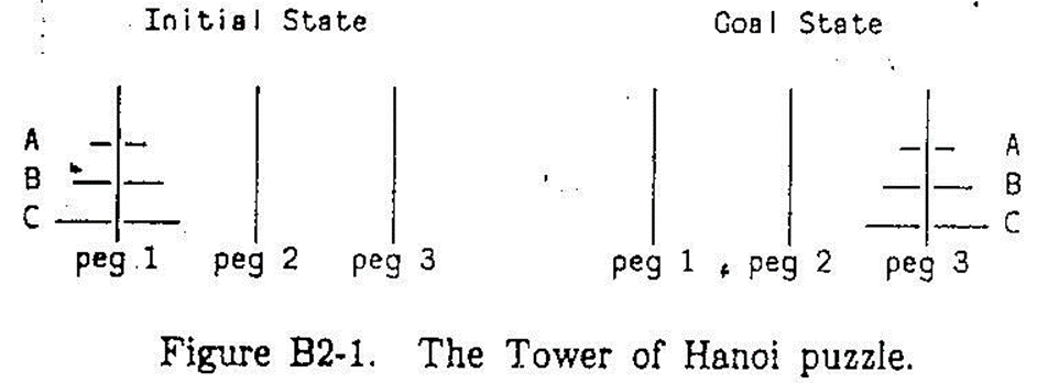
Only 1 operator:
Given distinct pegs i, j and k, moving a stack of size n>1 from peg i to peg k can be replaced by the 3 sub-problems:
Moving a stack of size n-1 from i to j
Moving a stack of size 1 from i to k
Moving a stack of size n-1 from j to k
Primitive problem:
Moving a single disk from one peg to another, provided that no smaller disk is on the receiving peg. Otherwise problem unsolvable.
AND/OR Graph
Each node represents either a single problem or a set of problems to be solved.
The start node correspond to the original problem
a node representing a primitive problem, called a terminal node, has no descendants
P is reduced to sub-problem set A, B, C
If P can be solved if any one of sets A, B, or C can be solved, A, B, C are called OR nodes.
If P can be solved only if all its members can be solved, they are called AND nodes.
The arcs leading to AND-node successors of a common parent are joined by a horizontal line.Example: (robot planning)
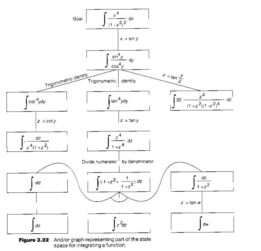
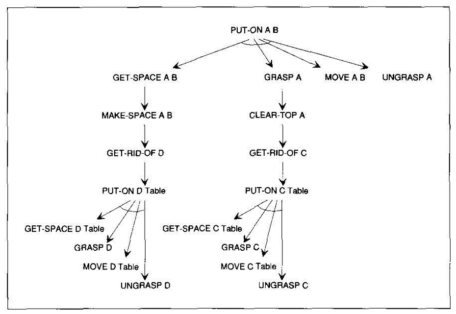
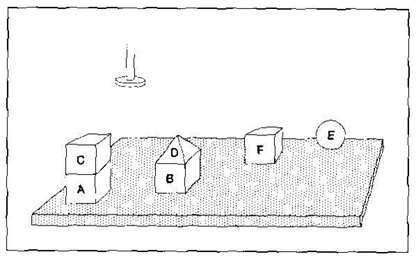
A node is solvable if
It is a terminal node (a primitive problem)
It is a non-terminal node whose successors are AND nodes that are all solvable, or
It is a non-terminal node whose successors are OR nodes and at least one of them is solvable.
Game Tree
a representation of all possible plays of a game.
Root node 0 initial state (the 1st player's turn to move)
Successors 0 states he can reach in one move
Their successors are the other player's possible reply.
Terminal node 0 configuration representing win, loss or draw
Each path from the root node to a terminal node gives a different complete play of the game.
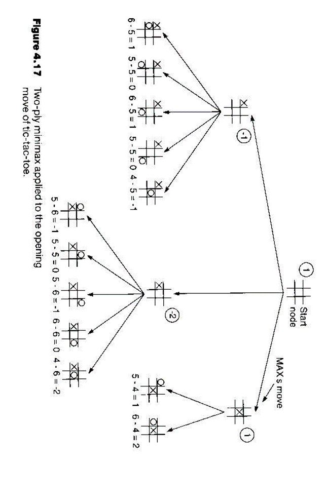
Example (tic-tac-toe)
Search Strategies
Blind State-Space Search
Do not use any domain specific information to assist the search.
Assumption made:
There is a procedure called expand for finding all successors of a given node.
The state space is a tree (can convert a graph into a tree with repeated nodes)
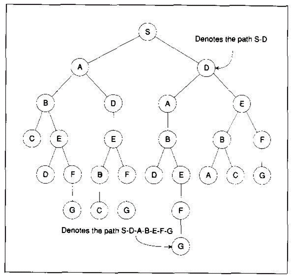
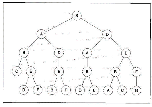
Breadth-first search
Expand nodes in order of their proximity to the start node, measured by the no. Of arcs between them.
Algorithms:
Put the start node on a list, called OPEN, of unexpanded nodes. If the start node is a goal node, a solution is found.
If OPEN is empty, no solution exists
Remove the first node, n, from OPEN and place it in a list, called CLOSED, of expanded nodes
Expand node n. If it has no successors, goto 2.
Place all successors of node n at the end of the OPEN list.
If any of the successors of node n is a goal node, a solution has been found. Otherwise goto 2.
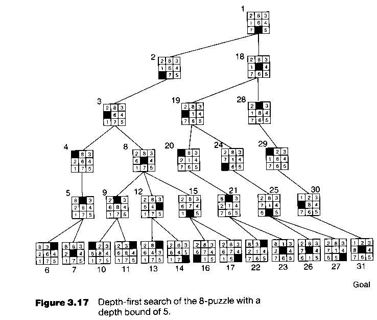
2. Depth-first search
Characterized by the expansion of the most recently generated, or deepest node first, where the depth of a node is defined as:
start node: depth 0
other nodes: depth of its predecessor + 1
Note that in many problems, the state-space tree may be of infinite depth. A maximum is often placed on the depth of nodes to be expanded.
Algorithms
Put the start node on a list, OPEN, of unexpanded nodes. If it is a goal node, a solution has been found.
If OPEN is empty, no solution exists.
Move the first node, n, on OPEN to a list, CLOSED of expanded nodes.
If the depth of node n is equal to the max depth, goto 2.
Expand node n. If it has no successor, goto 2.
Place all successors of node n at the beginning of OPEN.
If any of the successors of node n is a goal node, a solution has been found. Otherwise, goto 2.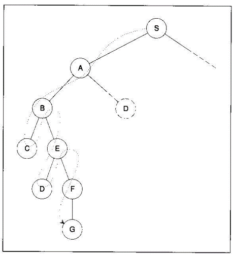
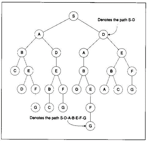


 Example:
Traces of searches:
Breadth-first search:
- Open=[S]; closed=[]
- Open=[A,D]; closed=[S]
- Open=[D,B,D]; closed=[S,A]
- Open=[B,D,A,E]; closed=[S,A,D]
- Open=[D,A,E,C,E]; closed=[S,A,D,B]
- ...
Depth-first search:
- Open=[S]; closed=[]
- Open=[A,D]; closed=[S]
- Open=[B,D,D]; closed=[S,A]
- Open=[C,E,D,D]; closed=[S,A,B]
- Open=[E,D,D]; closed=[S,A,B,C]
- Open=[D,F,D,D]; closed=[S,A,B,C,E]
- ...
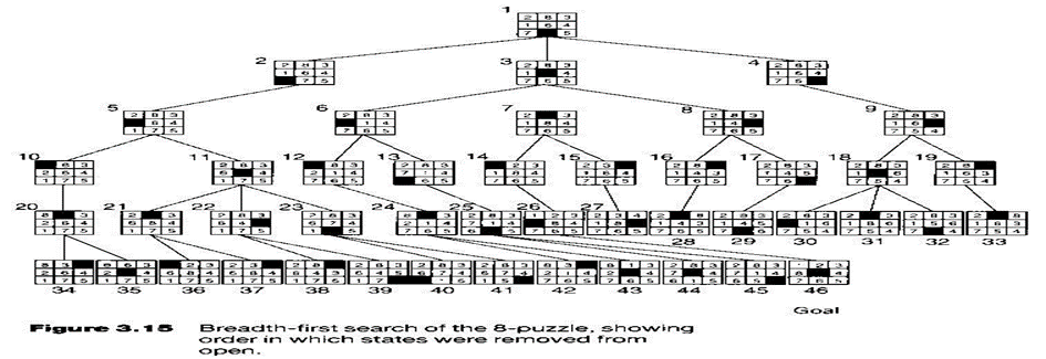
8-puzzle:
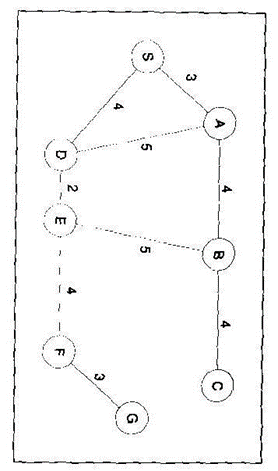
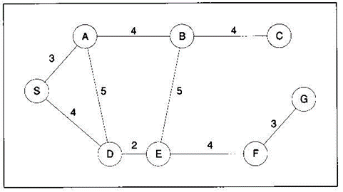
Uniform-cost Search
Generalized to find the cheapest path from the start node to the goal node.
A non-negative cost is associated with every arc joining two nodes. Cost of solution path=sum of arc costs along the path.
If all arcs have equal cost 0 breadth-first search
Let c(i,j) = cost of arc from node i to node j.
g(i) = cost of a path from start node to node i
Algorithm:
Put the start node S on a list called OPEN, of unexpanded nodes. If the start node is a goal node, a solution has been found. Otherwise, set g(s)=0.
If OPEN is empty, no solution exists.
Select from OPEN a node i such that g(i) is minimum. If several nodes qualify, choose node i to be a goal node if there is one; otherwise, choose among them arbitrarily. Move node i from OPEN to a list CLOSED of expanded nodes.
If node i is a goal node, a solution has been found.
Expand node i. If there is no successor, goto 2.
For each successor node j of node i, compute
g(j) = g(i) + c(i,j)
and place all successor nodes j in OPEN.
Goto 2.
Search Result
(value of g(x) is in parenthesis)
OPEN=[S(0)]; CLOSED=[]
OPEN=[A(3), D(4)]; CLOSED=[S]
OPEN=[B(7), D(8), D(4)]; CLOSED=[S,A]
OPEN=[B(7), D(8), A(9), E(6)]; CLOSED=[S,A,D]
OPEN=[B(7), D(8), A(9), B(11), F(10)]; CLOSED=[S,A,D,E]
...
Bi-directional Search
Search is likely to grow exponentially with the no. Of search levels.
Combine forward and backward search. Replace a single search graph by two smaller graphs (the number of level will be halved), one starting from start node, the other from goal node.
Search will terminate when two graphs intersect.
Empirical studies show that bi-directional search expands only ~1/4 as many nodes as uni-directional search.
Only applicable if we can expand backwards.
Notations:
s=start node, t=goal node.
S-OPEN and S-CLOSED are lists of unexpanded and expanded nodes respectively, generated from start node.
T-OPEN and T-CLOSED are lists of unexpanded and exapned nodes, respectively, generated from goal node.
Cost from node n to node x: c(n,x)
Gs(x) = shortest path so far from s to x
Gt(x) = shortest path so far from x to t
Algorithm:
Put s in S-CLOSED, with gs(s)=0. Expand node s. For each successor node x, place x on S-OPEN and set gs(x) to c(s,x).
Correspondingly, put t in T-CLOSED with gt(t)=0. Expand node t. For each predecessor node x, place x in T-OPEN and set gt(x) to c(x,t).
Decide whether to go forward or backward, e.g. (1) alternate between forward & backward, or (2) move backward if T-OPEN contains fewer nodes than S-OPEN, otherwise forward.
If forward, goto (3), else goto (4).
Select from S-OPEN a node n at which gs(n) is minimum. Move n to S-CLOSED. If n is also in T-CLOSED, goto (5). Otherwise, for each successor x of n:
If x is on neither S-OPEN nor S-CLOSED, then add x to S-OPEN. Gs(x) = gs(n) + c(n,x)
If x was already on S-OPEN, a shorter path to x may have just been found. Compare the previous cost gs(x) with gs(n)+c(n,x). If the latter is smaller, set gs(x) to the new path cost.
If x was already on S-CLOSED, do nothing (even though a new path to x has been found, its cost must be at least as great as the cost of the path already known)
Return to (2).
Select from T-OPEN a node at which gt(n) is min. Move n to T-CLOSED. If n is also in S-CLOSED, goto (5). Otherwise, for each predecessor x of n:
If x is on neither T-OPEN nor T-CLOSED, then add it to T-OPEN. Set gt(x) = gt(n) + c(x,n)
If x was already on T-OPEN and a shorter path from x to t has just been found, set gt(x) to the new value.
If x was already in T-CLOSED, do nothing.
Return to (2).
Consider the set of nodes that are in both S-CLOSED and either T-CLOSED or T-OPEN. Select from this set a node n for which gs(n)+gt(n) is minimum.
Non-deterministic Search
Expand a node chosen at random.
Algorithm:
Put the start node s on a list called OPEN of unexpanded nodes. If the start node is a goal node, a solution has been found.
If OPEN is empty, no solution exists
Remove the first node n from OPEN and place it in a list, called CLOSED, of expanded nodes.
Expand node n. If it has no successors, goto 2.
Place all successors of node n at random places in the OPEN list.
If any of the successors of node n is a goal node, a solution has been found. Otherwise, goto 2.
Blind AND/OR Graph Search
Assumptions:
The search space is an AND/OR tree and not a general graph.
When a problem is transformed to a set of sub-problems, the sub-problems may be solved in any order.
Breadth-first search
Put the start node on a list OPEN of unexpanded nodes.
Remove the first node n from OPEN.
Expand node n, generating all its immediate successor, and for each successor m, if m represents a set of more than one sub-problem, generate successors of m corresponding to the individual sub-problems. Attached to each newly generated node, a pointer back to its immediate predecessor. Place all the new nodes that do not yet have descendants at the end of OPEN.
If no successors were generated in (3), then
Label node n solvable
If the unsolvability of n makes any of its ancestors unsolvable, label these unsolvable.
If the start node is labeled unsolvable, exit
Remove from OPEN any nodes with an unsolvable ancestors.
Otherwise, if any terminal nodes were generated in (3),
Label these nodes solved.
If the solution of these terminal nodes makes any of their ancestors solved, label them solved.
If start node is labeled solved, exit
Remove from OPEN any nodes that are labeled solved, or that have a solved ancestor.
Goto 2.
Depth-first search
By chaning step (3) of previous algorithm:
If the depth of n is less than the depth bound, then expand node n, generating all its immediate successors and for each successor m, if m represents a set of more than one sub-problem, generating successors of m corresponding to the individual sub-problems. Attach to each newly generated node, a pointer back to its immediate predecessor. Place all the new nodes that do not yet has descendants at the beginning of OPEN.
Example:
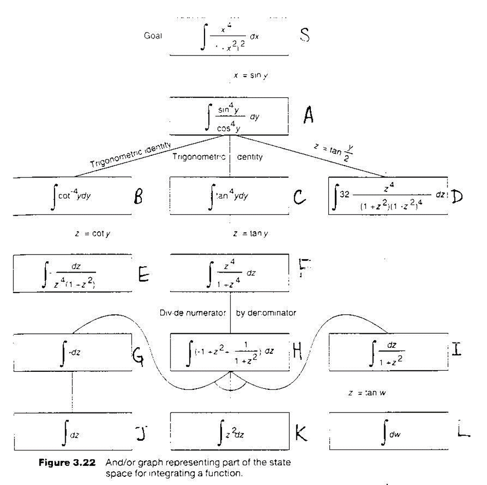
Breadth-first search:
OPEN | Unsolable | Solvable |
[S] |
|
|
[A] |
|
|
[B,C,D] |
|
|
[C,D,E] |
|
|
[D,E,F] |
|
|
[E,F] | D |
|
[F] | D,E,B |
|
[G,I] | D,E,B | K |
[I] | D,E,B | K,J,G |
[] | D,E,B | K,J,G,L,I,H,F, |
Depth-first search:
OPEN | Unsolvable | Solvable |
[S] |
|
|
[A] |
|
|
[B, C, D] |
|
|
[C, D] | E |
|
[F D] | E |
|
[G, I D] | E | K |
[I D] | E | K,J,G |
[D] | E | K,J,G,L,I,H |
PROBLEM REDUCTION:
So far we have considered search strategies for OR graphs through which we want to find a single path to a goal. Such structure represent the fact that we know how to get from anode to a goal state if we can discover how to get from that node to a goal state along any one of the branches leaving it.
AND-OR GRAPHS
The AND-OR GRAPH (or tree) is useful for representing the solution of problems that can solved by decomposing them into a set of smaller problems, all of which must then be solved. This decomposition, or reduction, generates arcs that we call AND arcs. One AND arc may point to any number of successor nodes, all of which must be solved in order for the arc to point to a solution. Just as in an OR graph, several arcs may emerge from a single node, indicating a variety of ways in which the original problem might be solved. This is why the structure is called not simply an AND-graph but rather an AND-OR graph (which also happens to be an AND-OR tree)
EXAMPLE FOR AND-OR GRAPH
ALGORITHM:
- Let G be a graph with only starting node INIT.
- Repeat the followings until INIT is labeled SOLVED or h(INIT) > FUTILITY
a) Select an unexpanded node from the most promising path from INIT (call it NODE)
b) Generate successors of NODE. If there are none, set h(NODE) = FUTILITY (i.e., NODE is unsolvable); otherwise for each SUCCESSOR that is not an ancestor of NODE do the following:
i. Add SUCCESSSOR to G.
Ii. If SUCCESSOR is a terminal node, label it SOLVED and set h(SUCCESSOR) = 0.
Iii. If SUCCESSPR is not a terminal node, compute its h
c) Propagate the newly discovered information up the graph by doing the following: let S be set of SOLVED nodes or nodes whose h values have been changed and need to have values propagated back to their parents. Initialize S to Node. Until S is empty repeat the followings:
i. Remove a node from S and call it CURRENT.
Ii. Compute the cost of each of the arcs emerging from CURRENT. Assign minimum cost of its successors as its h.
Iii. Mark the best path out of CURRENT by marking the arc that had the minimum cost in step ii
Iv. Mark CURRENT as SOLVED if all of the nodes connected to it through new labeled arc have been labeled SOLVED
v. If CURRENT has been labeled SOLVED or its cost was just changed, propagate its new cost back up through the graph. So add all of the ancestors of CURRENT to S.
EXAMPLE: 1
STEP 1:
A is the only node, it is at the end of the current best path. It is expanded, yielding nodes B, C, D. The arc to D is labeled as the most promising one emerging from A, since it costs 6compared to B and C, Which costs 9.
STEP 2:
Node B is chosen for expansion. This process produces one new arc, the AND arc to E and F, with a combined cost estimate of 10.so we update the f’ value of D to 10.Going back one more level, we see that this makes the AND arc B-C better than the arc to D, so it is labeled as the current best path.
STEP 3:
We traverse the arc from A and discover the unexpanded nodes B and C. If we going to find a solution along this path, we will have to expand both B and C eventually, so let’s choose to explore B first. This generates two new arcs, the ones to G and to H. Propagating their f’ values backward, we update f’ of B to 6(since that is the best we think we can do, which we can achieve by going through G). This requires updating the cost of the AND arc B-C to 12(6+4+2). After doing that, the arc to D is again the better path from A, so we record that as the current best path and either node E or node F will chose for expansion at step 4.
The Depth first search and Breadth first search given earlier for OR trees or graphs can be easily adopted by AND-OR graph. The main difference lies in the way termination conditions are determined, since all goals following an AND nodes must be realized; where as a single goal node following an OR node will do. So for this purpose we are using AO* algorithm.
Like A* algorithm here we will use two arrays and one heuristic function.
OPEN:
It contains the nodes that has been traversed but yet not been marked solvable or unsolvable.
CLOSE:
It contains the nodes that have already been processed.
6 7:The distance from current node to goal node.
Algorithm:
Step 1: Place the starting node into OPEN.
Step 2: Compute the most promising solution tree say T0.
Step 3: Select a node n that is both on OPEN and a member of T0. Remove it from OPEN and place it in
CLOSE
Step 4: If n is the terminal goal node then leveled n as solved and leveled all the ancestors of n as solved. If the starting node is marked as solved then success and exit.
Step 5: If n is not a solvable node, then mark n as unsolvable. If starting node is marked as unsolvable, then return failure and exit.
Step 6: Expand n. Find all its successors and find their h (n) value, push them into OPEN.
Step 7: Return to Step 2.
Step 8: Exit.
Implementation:
Let us take the following example to implement the AO* algorithm.
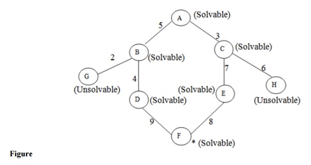
Step 1:
In the above graph, the solvable nodes are A, B, C, D, E, F and the unsolvable nodes are G, H. Take A as the starting node. So place A into OPEN.

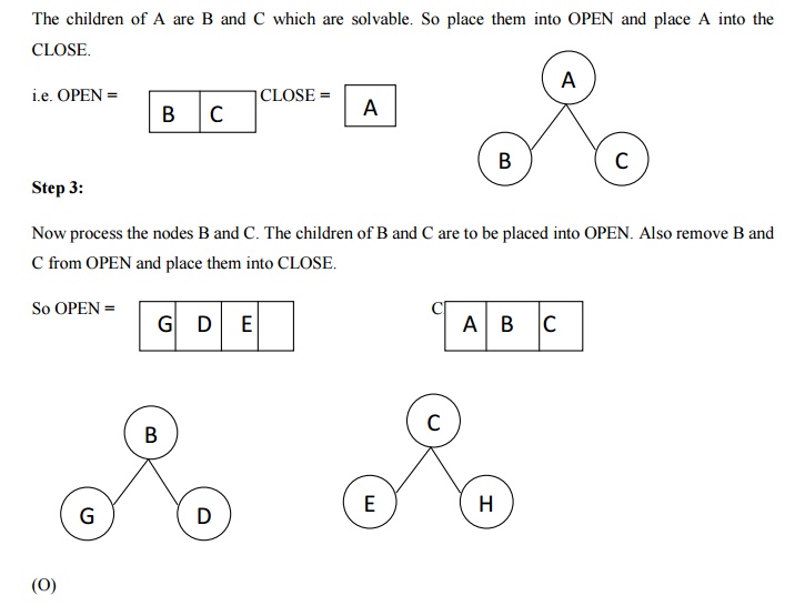
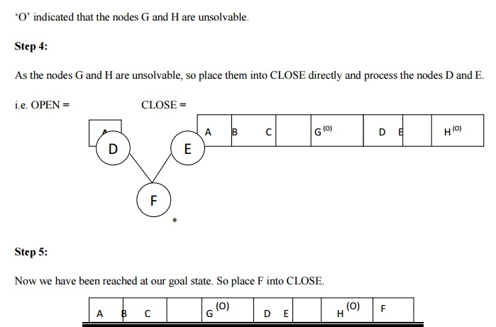
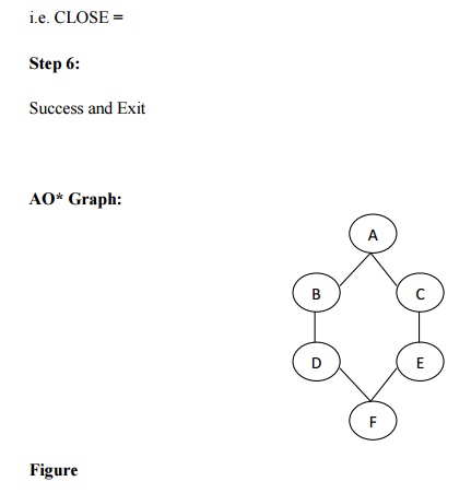
Advantages:
It is an optimal algorithm.
If traverse according to the ordering of nodes. It can be used for both OR and AND graph.
Disadvantages:
Sometimes for unsolvable nodes, it can’t find the optimal path. Its complexity is than other algorithms.
A constraint satisfaction problem (CSP) consists of
- a set of variables,
- a domain for each variable, and
- a set of constraints.
The aim is to choose a value for each variable so that the resulting possible world satisfies the constraints; we want a model of the constraints.
A finite CSP has a finite set of variables and a finite domain for each variable. Many of the methods considered in this chapter only work for finite CSPs, although some are designed for infinite, even continuous, domains.
The multidimensional aspect of these problems, where each variable can be seen as a separate dimension, makes them difficult to solve but also provides structure that can be exploited.
Given a CSP, there are a number of tasks that can be performed:
- Determine whether or not there is a model.
- Find a model.
- Find all of the models or enumerate the models.
- Count the number of models.
- Find the best model, given a measure of how good models are.
- Determine whether some statement holds in all models.
This chapter mostly considers the problem of finding a model. Some of the methods can also determine if there is no solution. What may be more surprising is that some of the methods can find a model if one exists, but they cannot tell us that there is no model if none exists.
CSPs are very common, so it is worth trying to find relatively efficient ways to solve them. Determining whether there is a model for a CSP with finite domains is NP-hard and no known algorithms exist to solve such problems that do not use exponential time in the worst case. However, just because a problem is NP-hard does not mean that all instances are difficult to solve. Many instances have structure that can be exploited.
- We have studied the strategies which can reason either in forward or backward, but a mixture of the two directions is appropriate for solving a complex and large problem. Such a mixed strategy, make it possible that first to solve the major part of a problem and then go back and solve the small problems arise during combining the big parts of the problem. Such a technique is called Means-Ends Analysis.
- Means-Ends Analysis is problem-solving techniques used in Artificial intelligence for limiting search in AI programs.
- It is a mixture of Backward and forward search technique.
- The MEA technique was first introduced in 1961 by Allen Newell, and Herbert A. Simon in their problem-solving computer program, which was named as General Problem Solver (GPS).
- The MEA analysis process centered on the evaluation of the difference between the current state and goal state.
How means-ends analysis Works:
The means-ends analysis process can be applied recursively for a problem. It is a strategy to control search in problem-solving. Following are the main Steps which describes the working of MEA technique for solving a problem.
- First, evaluate the difference between Initial State and final State.
- Select the various operators which can be applied for each difference.
- Apply the operator at each difference, which reduces the difference between the current state and goal state.
Operator Subgoaling
In the MEA process, we detect the differences between the current state and goal state. Once these differences occur, then we can apply an operator to reduce the differences. But sometimes it is possible that an operator cannot be applied to the current state. So we create the subproblem of the current state, in which operator can be applied, such type of backward chaining in which operators are selected, and then sub goals are set up to establish the preconditions of the operator is called Operator Subgoaling.
Algorithm for Means-Ends Analysis:
Let's we take Current state as CURRENT and Goal State as GOAL, then following are the steps for the MEA algorithm.
- Step 1: Compare CURRENT to GOAL, if there are no differences between both then return Success and Exit.
- Step 2: Else, select the most significant difference and reduce it by doing the following steps until the success or failure occurs.
- Select a new operator O which is applicable for the current difference, and if there is no such operator, then signal failure.
- Attempt to apply operator O to CURRENT. Make a description of two states.
i) O-Start, a state in which O?s preconditions are satisfied.
ii) O-Result, the state that would result if O were applied In O-start. - If
(First-Part <------ MEA (CURRENT, O-START)
And
(LAST-Part <----- MEA (O-Result, GOAL), are successful, then signal Success and return the result of combining FIRST-PART, O, and LAST-PART.
The above-discussed algorithm is more suitable for a simple problem and not adequate for solving complex problems.
Example of Mean-Ends Analysis:
Let's take an example where we know the initial state and goal state as given below. In this problem, we need to get the goal state by finding differences between the initial state and goal state and applying operators.
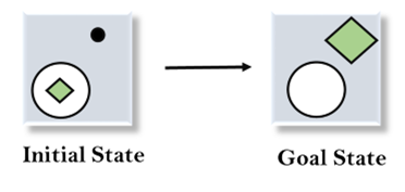
Solution:
To solve the above problem, we will first find the differences between initial states and goal states, and for each difference, we will generate a new state and will apply the operators. The operators we have for this problem are:
- Move
- Delete
- Expand
1. Evaluating the initial state: In the first step, we will evaluate the initial state and will compare the initial and Goal state to find the differences between both states.

2. Applying Delete operator: As we can check the first difference is that in goal state there is no dot symbol which is present in the initial state, so, first we will apply the Delete operator to remove this dot.
3. Applying Move Operator: After applying the Delete operator, the new state occurs which we will again compare with goal state. After comparing these states, there is another difference that is the square is outside the circle, so, we will apply the Move Operator.

4. Applying Expand Operator: Now a new state is generated in the third step, and we will compare this state with the goal state. After comparing the states there is still one difference which is the size of the square, so, we will apply Expand operator, and finally, it will generate the goal state.

What Does “Stochastic” Mean?
A variable is stochastic if the occurrence of events or outcomes involves randomness or uncertainty.
… “stochastic” means that the model has some kind of randomness in it
A process is stochastic if it governs one or more stochastic variables.
Games are stochastic because they include an element of randomness, such as shuffling or rolling of a dice in card games and board games.
In real life, many unpredictable external events can put us into unforeseen situations. Many games mirror this unpredictability by including a random element, such as the throwing of dice. We call these stochastic games.
Stochastic is commonly used to describe mathematical processes that use or harness randomness. Common examples include Brownian motion, Markov Processes, Monte Carlo Sampling, and more.
Now that we have some definitions, let’s try and add some more context by comparing stochastic with other notions of uncertainty.
Stochastic vs. Random, Probabilistic, and Non-deterministic
In this section, we’ll try to better understand the idea of a variable or process being stochastic by comparing it to the related terms of “random,” “probabilistic,” and “non-deterministic.”
Stochastic vs. Random
In statistics and probability, a variable is called a “random variable” and can take on one or more outcomes or events.
It is the common name used for a thing that can be measured.
In general, stochastic is a synonym for random.
For example, a stochastic variable is a random variable. A stochastic process is a random process.
Typically, random is used to refer to a lack of dependence between observations in a sequence. For example, the rolls of a fair die are random, so are the flips of a fair coin.
Strictly speaking, a random variable or a random sequence can still be summarized using a probability distribution; it just may be a uniform distribution.
We may choose to describe something as stochastic over random if we are interested in focusing on the probabilistic nature of the variable, such as a partial dependence of the next event on the current event. We may choose random over stochastic if we wish to focus attention on the independence of the events.
Stochastic vs. Probabilistic
In general, stochastic is a synonym for probabilistic.
For example, a stochastic variable or process is probabilistic. It can be summarized and analyzed using the tools of probability.
Most notably, the distribution of events or the next event in a sequence can be described in terms of a probability distribution.
We may choose to describe a variable or process as probabilistic over stochastic if we wish to emphasize the dependence, such as if we are using a parametric model or known probability distribution to summarize the variable or sequence.
Stochastic vs. Non-deterministic
A variable or process is deterministic if the next event in the sequence can be determined exactly from the current event.
For example, a deterministic algorithm will always give the same outcome given the same input. Conversely, a non-deterministic algorithm may give different outcomes for the same input.
A stochastic variable or process is not deterministic because there is uncertainty associated with the outcome.
Nevertheless, a stochastic variable or process is also not non-deterministic because non-determinism only describes the possibility of outcomes, rather than probability.
Describing something as stochastic is a stronger claim than describing it as non-deterministic because we can use the tools of probability in analysis, such as expected outcome and variance.
… “stochastic” generally implies that uncertainty about outcomes is quantified in terms of probabilities; a nondeterministic environment is one in which actions are characterized by their possible outcomes, but no probabilities are attached to them.
Stochastic in Machine Learning
Many machine learning algorithms and models are described in terms of being stochastic.
This is because many optimization and learning algorithms both must operate in stochastic domains and because some algorithms make use of randomness or probabilistic decisions.
Let’s take a closer look at the source of uncertainty and the nature of stochastic algorithms in machine learning.
Stochastic Problem Domains
Stochastic domains are those that involve uncertainty.
… machine learning must always deal with uncertain quantities, and sometimes may also need to deal with stochastic (non-deterministic) quantities. Uncertainty and stochasticity can arise from many sources.
This uncertainty can come from a target or objective function that is subjected to statistical noise or random errors.
It can also come from the fact that the data used to fit a model is an incomplete sample from a broader population.
Finally, the models chosen are rarely able to capture all of the aspects of the domain, and instead must generalize to unseen circumstances and lose some fidelity.
Stochastic Optimization Algorithms
Stochastic optimization refers to a field of optimization algorithms that explicitly use randomness to find the optima of an objective function, or optimize an objective function that itself has randomness (statistical noise).
Most commonly, stochastic optimization algorithms seek a balance between exploring the search space and exploiting what has already been learned about the search space in order to hone in on the optima. The choice of the next locations in the search space are chosen stochastically, that is probabilistically based on what areas have been searched recently.
Stochastic hill climbing chooses at random from among the uphill moves; the probability of selection can vary with the steepness of the uphill move.
Popular examples of stochastic optimization algorithms are:
- Simulated Annealing
- Genetic Algorithm
- Particle Swarm Optimization
Particle swarm optimization (PSO) is a stochastic optimization approach, modeled on the social behavior of bird flocks.
Stochastic Learning Algorithms
Most machine learning algorithms are stochastic because they make use of randomness during learning.
Using randomness is a feature, not a bug. It allows the algorithms to avoid getting stuck and achieve results that deterministic (non-stochastic) algorithms cannot achieve.
For example, some machine learning algorithms even include “stochastic” in their name such as:
- Stochastic Gradient Descent (optimization algorithm).
- Stochastic Gradient Boosting (ensemble algorithm).
Stochastic gradient descent optimizes the parameters of a model, such as an artificial neural network, that involves randomly shuffling the training dataset before each iteration that causes different orders of updates to the model parameters. In addition, model weights in a neural network are often initialized to a random starting point.
Most deep learning algorithms are based on an optimization algorithm called stochastic gradient descent.
Stochastic gradient boosting is an ensemble of decision trees algorithms. The stochastic aspect refers to the random subset of rows chosen from the training dataset used to construct trees, specifically the split points of trees.
Stochastic Algorithm Behaviour
Because many machine learning algorithms make use of randomness, their nature (e.g. Behavior and performance) is also stochastic.
The stochastic nature of machine learning algorithms is most commonly seen on complex and nonlinear methods used for classification and regression predictive modeling problems.
These algorithms make use of randomness during the process of constructing a model from the training data which has the effect of fitting a different model each time same algorithm is run on the same data. In turn, the slightly different models have different performance when evaluated on a hold out test dataset.
This stochastic behavior of nonlinear machine learning algorithms is challenging for beginners who assume that learning algorithms will be deterministic, e.g. Fit the same model when the algorithm is run on the same data.
This stochastic behavior requires that the performance of the model must be summarized using summary statistics that describe the mean or expected performance of the model, rather than the performance of the model from any single training run.
Problem : Given a cost function f: R^n –> R, find an n-tuple that minimizes the value of f. Note that minimizing the value of a function is algorithmically equivalent to maximization (since we can redefine the cost function as 1-f).
Many of you with a background in calculus/analysis are likely familiar with simple optimization for single variable functions. For instance, the function f(x) = x^2 + 2x can be optimized setting the first derivative equal to zero, obtaining the solution x = -1 yielding the minimum value f(-1) = -1. This technique suffices for simple functions with few variables. However, it is often the case that researchers are interested in optimizing functions of several variables, in which case the solution can only be obtained computationally.
One excellent example of a difficult optimization task is the chip floor planning problem. Imagine you’re working at Intel and you’re tasked with designing the layout for an integrated circuit. You have a set of modules of different shapes/sizes and a fixed area on which the modules can be placed. There are a number of objectives you want to achieve: maximizing ability for wires to connect components, minimize net area, minimize chip cost, etc. With these in mind, you create a cost function, taking all, say, 1000 variable configurations and returning a single real value representing the ‘cost’ of the input configuration. We call this the objective function, since the goal is to minimize its value.
A naive algorithm would be a complete space search — we search all possible configurations until we find the minimum. This may suffice for functions of few variables, but the problem we have in mind would entail such a brute force algorithm to fun in O(n!).
Due to the computational intractability of problems like these, and other NP-hard problems, many optimization heuristics have been developed in an attempt to yield a good, albeit potentially suboptimal, value. In our case, we don’t necessarily need to find a strictly optimal value — finding a near-optimal value would satisfy our goal. One widely used technique is simulated annealing, by which we introduce a degree of stochasticity, potentially shifting from a better solution to a worse one, in an attempt to escape local minima and converge to a value closer to the global optimum.
Simulated annealing is based on metallurgical practices by which a material is heated to a high temperature and cooled. At high temperatures, atoms may shift unpredictably, often eliminating impurities as the material cools into a pure crystal. This is replicated via the simulated annealing optimization algorithm, with energy state corresponding to current solution.
In this algorithm, we define an initial temperature, often set as 1, and a minimum temperature, on the order of 10^-4. The current temperature is multiplied by some fraction alpha and thus decreased until it reaches the minimum temperature. For each distinct temperature value, we run the core optimization routine a fixed number of times. The optimization routine consists of finding a neighboring solution and accepting it with probability e^(f(c) – f(n)) where c is the current solution and n is the neighboring solution. A neighboring solution is found by applying a slight perturbation to the current solution. This randomness is useful to escape the common pitfall of optimization heuristics — getting trapped in local minima. By potentially accepting a less optimal solution than we currently have, and accepting it with probability inverse to the increase in cost, the algorithm is more likely to converge near the global optimum. Designing a neighbor function is quite tricky and must be done on a case by case basis, but below are some ideas for finding neighbors in locational optimization problems.
- Move all points 0 or 1 units in a random direction
- Shift input elements randomly
- Swap random elements in input sequence
- Permute input sequence
- Partition input sequence into a random number of segments and permute segments
One caveat is that we need to provide an initial solution so the algorithm knows where to start. This can be done in two ways: (1) using prior knowledge about the problem to input a good starting point and (2) generating a random solution. Although generating a random solution is worse and can occasionally inhibit the success of the algorithm, it is the only option for problems where we know nothing about the landscape.
There are many other optimization techniques, although simulated annealing is a useful, stochastic optimization heuristic for large, discrete search spaces in which optimality is prioritized over time. Below, I’ve included a basic framework for locational-based simulated annealing (perhaps the most applicable flavor of optimization for simulated annealing). Of course, the cost function, candidate generation function, and neighbor function must be defined based on the specific problem at hand, although the core optimization routine has already been implemented.
// Java program to implement Simulated Annealing Import java.util.*;
Public class SimulatedAnnealing {
// Initial and final temperature Public static double T = 1;
// Simulated Annealing parameters
// Temperature at which iteration terminates Static final double Tmin = .0001;
// Decrease in temperature Static final double alpha = 0.9;
// Number of iterations of annealing // before decreasing temperature Static final int numIterations = 100;
// Locational parameters
// Target array is discretized as M*N grid Static final int M = 5, N = 5;
// Number of objects desired Static final int k = 5;
Public static void main(String[] args) {
// Problem: place k objects in an MxN target // plane yielding minimal cost according to // defined objective function
// Set of all possible candidate locations String[][] sourceArray = new String[M][N];
// Global minimum Solution min = new Solution(Double.MAX_VALUE, null);
// Generates random initial candidate solution // before annealing process Solution currentSol = genRandSol();
// Continues annealing until reaching minimum // temprature While (T > Tmin) { For (int i=0;i<numIterations;i++){
// Reassigns global minimum accordingly If (currentSol.CVRMSE < min.CVRMSE){ Min = currentSol; }
Solution newSol = neighbor(currentSol); Double ap = Math.pow(Math.E, (currentSol.CVRMSE - newSol.CVRMSE)/T); If (ap > Math.random()) CurrentSol = newSol; }
T *= alpha; // Decreases T, cooling phase }
//Returns minimum value based on optimiation System.out.println(min.CVRMSE+"\n\n");
For(String[] row:sourceArray) Arrays.fill(row, "X");
// Displays For (int object:min.config) { Int[] coord = indexToPoints(object); SourceArray[coord[0]][coord[1]] = "-"; }
// Displays optimal location For (String[] row:sourceArray) System.out.println(Arrays.toString(row));
}
// Given current configuration, returns "neighboring" // configuration (i.e. very similar) // integer of k points each in range [0, n) /* Different neighbor selection strategies: * Move all points 0 or 1 units in a random direction * Shift input elements randomly * Swap random elements in input sequence * Permute input sequence * Partition input sequence into a random number Of segments and permute segments */ Public static Solution neighbor(Solution currentSol){
// Slight perturbation to the current solution // to avoid getting stuck in local minimas
// Returning for the sake of compilation Return currentSol;
}
// Generates random solution via modified Fisher-Yates // shuffle for first k elements // Pseudorandomly selects k integers from the interval // [0, n-1] Public static Solution genRandSol(){
// Instantiating for the sake of compilation Int[] a = {1, 2, 3, 4, 5};
// Returning for the sake of compilation Return new Solution(-1, a); }
// Complexity is O(M*N*k), asymptotically tight Public static double cost(int[] inputConfiguration){
// Given specific configuration, return object // solution with assigned cost Return -1; //Returning for the sake of compilation }
// Mapping from [0, M*N] --> [0,M]x[0,N] Public static int[] indexToPoints(int index){ Int[] points = {index%M, index/M}; Return points; }
// Class solution, bundling configuration with error Static class Solution {
// function value of instance of solution; // using coefficient of variance root mean // squared error Public double CVRMSE;
Public int[] config; // Configuration array Public Solution(double CVRMSE, int[] configuration) { This.CVRMSE = CVRMSE; Config = configuration; } } } |
Output :
-1.0
[X, -, X, X, X]
[-, X, X, X, X]
[-, X, X, X, X]
[-, X, X, X, X]
[-, X, X, X, X]
Particle Swarm Optimization characterized into the domain of Artificial inteligence. The term ‘Artificial Intelligence’ or ‘Artificial Life‘ refers to the theory of simulating human behavior through computation. It involves designing such computer systems which are able to execute tasks which require human intelligence. For eg, earlier only humans had the power to recognize the speech of a person. But now, speech recognition is a common feature of any digital device. This has become possible through artificial intelligence. Other examples of human intelligence may include decision making, language translation, and visual perception etc. There are various techniques which make it possible. These techniques to implement artificial intelligence into computers are popularly known as approaches of artificial intelligence’.
These techniques are designed basis two categories:
- The first study includes how biological phenomena can be studies using computation.
- The second one shows how biological phenomena can help understand computation problems. While studying the PSO Technique, we deal with in the second category.
There are three approaches of the artificial intelligence:
- Statistical Methods
- Symbolic Artificial Intelligence
- Computational Intelligence
Computational Intelligence can be implemented using either of the three methods:
- Artificial Neural Network
- Fuzzy Logic
- Evolutionary Computation
Note: Under Evolutionary Computation, are the Swarm Intelligence Techniques which include Particle Swarm Optimization.
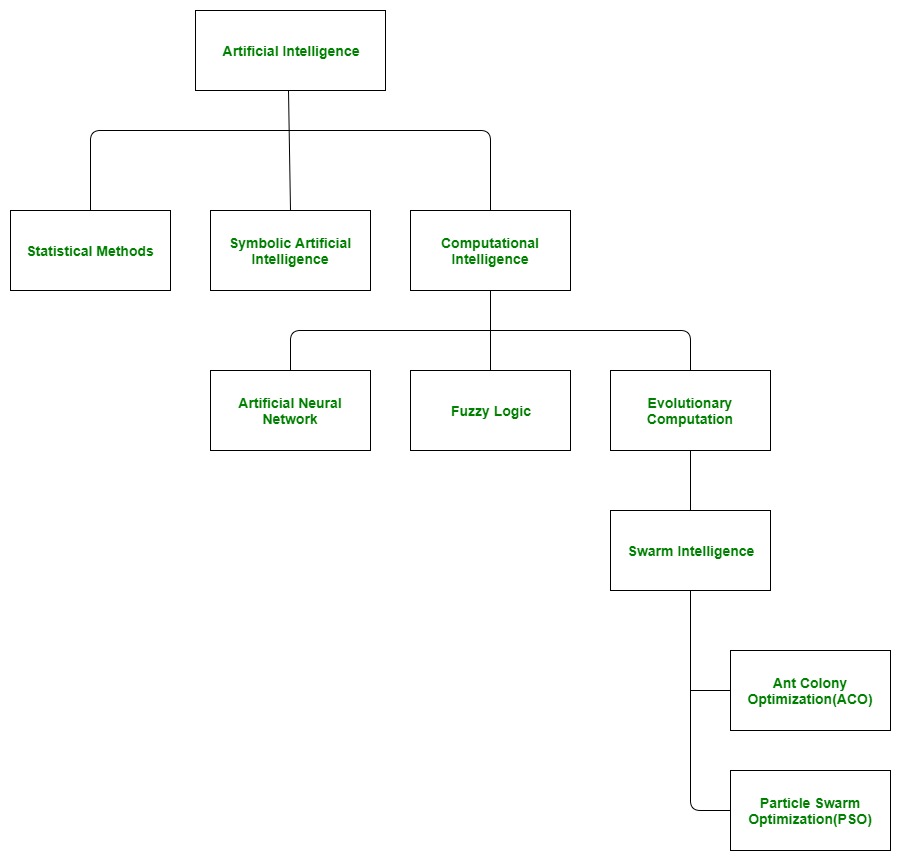
Concept of Particle Swarm Optimization
As described earlier, Swarm Intelligence is a branch of Artificial Intelligence where we observe nature and try to learn how different biological phenomena can be imitated in a computer system to optimize the scheduling algorithms. In swarm intelligence, we focus on the collective behavior of simple organisms and their interaction with the environment.
There are two types of Optimization algorithms in Swarm Intelligence:
- The first one is Ant Colony Optimization(ACO). Here the algorithm is based on the collective behavior of ants in their colony.
- The second technique is Particle Swarm Optimization(PSO).
In PSO, the focus in on a group of birds. This group of birds is referred to as a ‘swarm‘. Let’s try to understand the Particle Swarm Optimization from the following scenario.
Example: Suppose there is a swarm (a group of birds). Now, all the birds are hungry and are searching for food. These hungry birds can be correlated with the tasks in a computation system which are hungry for resources. Now, in the locality of these birds, there is only one food particle. This food particle can be correlated with a resource. As we know, tasks are many, resources are limited. So this has become a similar condition as in a certain computation environment. Now, the birds don’t know where the food particle is hidden or located. In such a scenario, how the algorithm to find the food particle should be designed. If every bird will try to find the food on its own, it may cause havoc and may consume a large amount of time. Thus on careful observation of this swarm, it was realized that though the birds don’t know where the food particle is located, they do know their distance from it. Thus the best approach to finding that food particle is to follow the birds which are nearest to the food particle. This behavior of birds is simulated in the computation environment and the algorithm so designed is termed as Particle Swarm Optimization Algorithm.
Note: This same behavior is also executed by a fish school. Thus Particle Swarm Optimization Technique is said to be inspired by a swarm of birds or a school of fish. Thus, this algorithm is also called a population-based stochastic algorithm and was developed by Dr. Russell C. Eberhart and Dr. James Kennedy in the year 1995.
This is the overall concept of what a particle swarm optimization is, and on what biological phenomena, its working is based upon.
- Mini-max algorithm is a recursive or backtracking algorithm which is used in decision-making and game theory. It provides an optimal move for the player assuming that opponent is also playing optimally.
- Mini-Max algorithm uses recursion to search through the game-tree.
- Min-Max algorithm is mostly used for game playing in AI. Such as Chess, Checkers, tic-tac-toe, go, and various tow-players game. This Algorithm computes the minimax decision for the current state.
- In this algorithm two players play the game, one is called MAX and other is called MIN.
- Both the players fight it as the opponent player gets the minimum benefit while they get the maximum benefit.
- Both Players of the game are opponent of each other, where MAX will select the maximized value and MIN will select the minimized value.
- The minimax algorithm performs a depth-first search algorithm for the exploration of the complete game tree.
- The minimax algorithm proceeds all the way down to the terminal node of the tree, then backtrack the tree as the recursion.
Pseudo-code for MinMax Algorithm:
- Function minimax(node, depth, maximizingPlayer) is
- If depth ==0 or node is a terminal node then
- Return static evaluation of node
- If MaximizingPlayer then // for Maximizer Player
- MaxEva= -infinity
- For each child of node do
- Eva= minimax(child, depth-1, false)
- MaxEva= max(maxEva,eva) //gives Maximum of the values
- Return maxEva
- Else // for Minimizer player
- MinEva= +infinity
- For each child of node do
- Eva= minimax(child, depth-1, true)
- MinEva= min(minEva, eva) //gives minimum of the values
- Return minEva
Initial call:
Minimax(node, 3, true)
Working of Min-Max Algorithm:
- The working of the minimax algorithm can be easily described using an example. Below we have taken an example of game-tree which is representing the two-player game.
- In this example, there are two players one is called Maximizer and other is called Minimizer.
- Maximizer will try to get the Maximum possible score, and Minimizer will try to get the minimum possible score.
- This algorithm applies DFS, so in this game-tree, we have to go all the way through the leaves to reach the terminal nodes.
- At the terminal node, the terminal values are given so we will compare those value and backtrack the tree until the initial state occurs. Following are the main steps involved in solving the two-player game tree:
Step-1: In the first step, the algorithm generates the entire game-tree and apply the utility function to get the utility values for the terminal states. In the below tree diagram, let's take A is the initial state of the tree. Suppose maximizer takes first turn which has worst-case initial value =- infinity, and minimizer will take next turn which has worst-case initial value = +infinity.
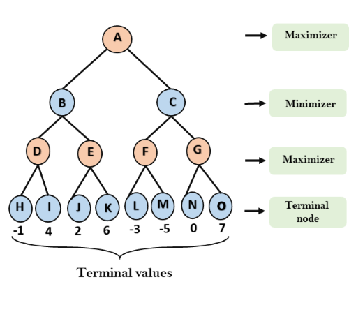
Step 2: Now, first we find the utilities value for the Maximizer, its initial value is -∞, so we will compare each value in terminal state with initial value of Maximizer and determines the higher nodes values. It will find the maximum among the all.
- For node D max(-1,- -∞) => max(-1,4)= 4
- For Node E max(2, -∞) => max(2, 6)= 6
- For Node F max(-3, -∞) => max(-3,-5) = -3
- For node G max(0, -∞) = max(0, 7) = 7
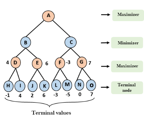
Step 3: In the next step, it's a turn for minimizer, so it will compare all nodes value with +∞, and will find the 3rd layer node values.
- For node B= min(4,6) = 4
- For node C= min (-3, 7) = -3
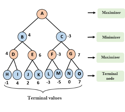
Step 3: Now it's a turn for Maximizer, and it will again choose the maximum of all nodes value and find the maximum value for the root node. In this game tree, there are only 4 layers, hence we reach immediately to the root node, but in real games, there will be more than 4 layers.
- For node A max(4, -3)= 4
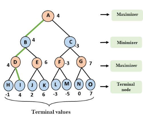
That was the complete workflow of the minimax two player game.
Properties of Mini-Max algorithm:
- Complete- Min-Max algorithm is Complete. It will definitely find a solution (if exist), in the finite search tree.
- Optimal- Min-Max algorithm is optimal if both opponents are playing optimally.
- Time complexity- As it performs DFS for the game-tree, so the time complexity of Min-Max algorithm is O(bm), where b is branching factor of the game-tree, and m is the maximum depth of the tree.
- Space Complexity- Space complexity of Mini-max algorithm is also similar to DFS which is O(bm).
Limitation of the minimax Algorithm:
The main drawback of the minimax algorithm is that it gets really slow for complex games such as Chess, go, etc. This type of games has a huge branching factor, and the player has lots of choices to decide. This limitation of the minimax algorithm can be improved from alpha-beta pruning which we have discussed in the next topic.
- Alpha-beta pruning is a modified version of the minimax algorithm. It is an optimization technique for the minimax algorithm.
- As we have seen in the minimax search algorithm that the number of game states it has to examine are exponential in depth of the tree. Since we cannot eliminate the exponent, but we can cut it to half. Hence there is a technique by which without checking each node of the game tree we can compute the correct minimax decision, and this technique is called pruning. This involves two threshold parameter Alpha and beta for future expansion, so it is called alpha-beta pruning. It is also called as Alpha-Beta Algorithm.
- Alpha-beta pruning can be applied at any depth of a tree, and sometimes it not only prune the tree leaves but also entire sub-tree.
- The two-parameter can be defined as:
- Alpha: The best (highest-value) choice we have found so far at any point along the path of Maximizer. The initial value of alpha is -∞.
- Beta: The best (lowest-value) choice we have found so far at any point along the path of Minimizer. The initial value of beta is +∞.
- The Alpha-beta pruning to a standard minimax algorithm returns the same move as the standard algorithm does, but it removes all the nodes which are not really affecting the final decision but making algorithm slow. Hence by pruning these nodes, it makes the algorithm fast.
Note: To better understand this topic, kindly study the minimax algorithm.
Condition for Alpha-beta pruning:
The main condition which required for alpha-beta pruning is:
- α>=β
Key points about alpha-beta pruning:
- The Max player will only update the value of alpha.
- The Min player will only update the value of beta.
- While backtracking the tree, the node values will be passed to upper nodes instead of values of alpha and beta.
- We will only pass the alpha, beta values to the child nodes.
Pseudo-code for Alpha-beta Pruning:
- Function minimax(node, depth, alpha, beta, maximizingPlayer) is
- If depth ==0 or node is a terminal node then
- Return static evaluation of node
- If MaximizingPlayer then // for Maximizer Player
- MaxEva= -infinity
- For each child of node do
- Eva= minimax(child, depth-1, alpha, beta, False)
- MaxEva= max(maxEva, eva)
- Alpha= max(alpha, maxEva)
- If beta<=alpha
- Break
- Return maxEva
- Else // for Minimizer player
- MinEva= +infinity
- For each child of node do
- Eva= minimax(child, depth-1, alpha, beta, true)
- MinEva= min(minEva, eva)
- Beta= min(beta, eva)
- If beta<=alpha
- Break
- Return minEva
Working of Alpha-Beta Pruning:
Let's take an example of two-player search tree to understand the working of Alpha-beta pruning
Step 1: At the first step the, Max player will start first move from node A where α= -∞ and β= +∞, these value of alpha and beta passed down to node B where again α= -∞ and β= +∞, and Node B passes the same value to its child D.
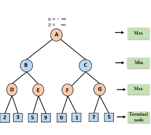
Step 2: At Node D, the value of α will be calculated as its turn for Max. The value of α is compared with firstly 2 and then 3, and the max (2, 3) = 3 will be the value of α at node D and node value will also 3.
Step 3: Now algorithm backtrack to node B, where the value of β will change as this is a turn of Min, Now β= +∞, will compare with the available subsequent nodes value, i.e. min (∞, 3) = 3, hence at node B now α= -∞, and β= 3.
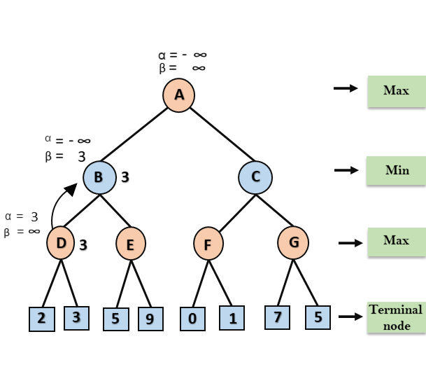
In the next step, algorithm traverse the next successor of Node B which is node E, and the values of α= -∞, and β= 3 will also be passed.
Step 4: At node E, Max will take its turn, and the value of alpha will change. The current value of alpha will be compared with 5, so max (-∞, 5) = 5, hence at node E α= 5 and β= 3, where α>=β, so the right successor of E will be pruned, and algorithm will not traverse it, and the value at node E will be 5.
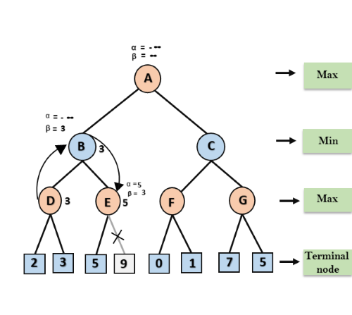
Step 5: At next step, algorithm again backtrack the tree, from node B to node A. At node A, the value of alpha will be changed the maximum available value is 3 as max (-∞, 3)= 3, and β= +∞, these two values now passes to right successor of A which is Node C.
At node C, α=3 and β= +∞, and the same values will be passed on to node F.
Step 6: At node F, again the value of α will be compared with left child which is 0, and max(3,0)= 3, and then compared with right child which is 1, and max(3,1)= 3 still α remains 3, but the node value of F will become 1.
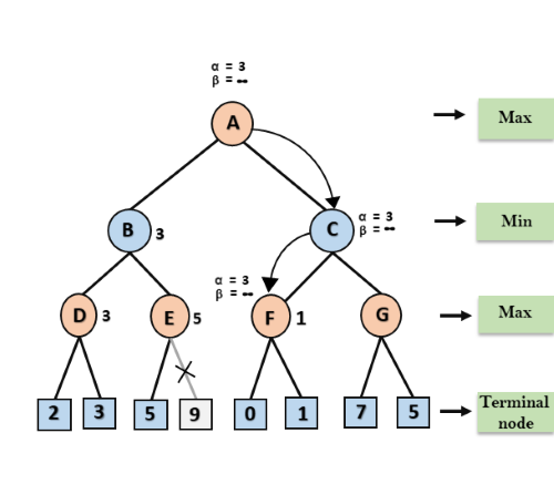
Step 7: Node F returns the node value 1 to node C, at C α= 3 and β= +∞, here the value of beta will be changed, it will compare with 1 so min (∞, 1) = 1. Now at C, α=3 and β= 1, and again it satisfies the condition α>=β, so the next child of C which is G will be pruned, and the algorithm will not compute the entire sub-tree G.
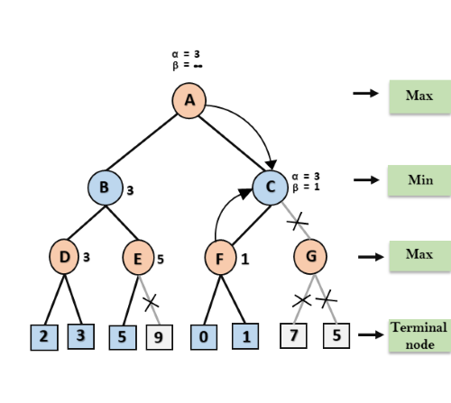
Step 8: C now returns the value of 1 to A here the best value for A is max (3, 1) = 3. Following is the final game tree which is the showing the nodes which are computed and nodes which has never computed. Hence the optimal value for the maximizer is 3 for this example.
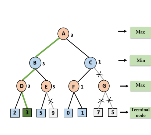
Move Ordering in Alpha-Beta pruning:
The effectiveness of alpha-beta pruning is highly dependent on the order in which each node is examined. Move order is an important aspect of alpha-beta pruning.
It can be of two types:
- Worst ordering: In some cases, alpha-beta pruning algorithm does not prune any of the leaves of the tree, and works exactly as minimax algorithm. In this case, it also consumes more time because of alpha-beta factors, such a move of pruning is called worst ordering. In this case, the best move occurs on the right side of the tree. The time complexity for such an order is O(bm).
- Ideal ordering: The ideal ordering for alpha-beta pruning occurs when lots of pruning happens in the tree, and best moves occur at the left side of the tree. We apply DFS hence it first search left of the tree and go deep twice as minimax algorithm in the same amount of time. Complexity in ideal ordering is O(bm/2).
Rules to find good ordering:
Following are some rules to find good ordering in alpha-beta pruning:
- Occur the best move from the shallowest node.
- Order the nodes in the tree such that the best nodes are checked first.
- Use domain knowledge while finding the best move. Ex: for Chess, try order: captures first, then threats, then forward moves, backward moves.
- We can bookkeep the states, as there is a possibility that states may repeat.
Text Books
1. S. Russell and P. Norvig, “Artificial Intelligence: A Modern Approach,” Prentice Hall
2. E. Rich, K. Knight and S. B. Nair, “Artificial Intelligence,” TMH
References
1. C. Bishop,“Pattern Recognition and Machine Learning," Springer
2. D. W. Patterson, “Introduction to artificial intelligence and expert systems,” Prentice Hall
3. A. C.Staugaard, Jr., “Robotics and AI: An Introduction to Applied Machine Intelligence,” Prentice Hall
4. I. Bratko, “Prolog Programming for Artificial Intelligence,” Addison-Wesley
5. S. O. Haykin, “Neural Networks and Learning Machines,” Prentice Hall
6. D.Jurafsky and J. H. Martin,“Speech and Language Processing,” Prentice Hall