UNIT 2

Knowledge And Reasoning

2.1 Knowledge and Reasoning: Building a knowledge base

• An intelligent agent needs knowledge about the real world for taking decisions and reasoning to act efficiently.
• Knowledge-based agents are those agents who have the capability of maintaining an internal state of knowledge, reason over that knowledge, update their knowledge after observations and take actions. These agents can represent the world with some formal representation and act intelligently.
• Knowledge-based agents are composed of two main parts:
  • Knowledge-base and
  • Inference system.

A knowledge-based agent must able to do the following:

• An agent should be able to represent states, actions, etc.
• An agent Should be able to incorporate new percepts
• An agent can update the internal representation of the world
• An agent can deduce the internal representation of the world
• An agent can deduce appropriate actions.

The architecture of knowledge-based agent:

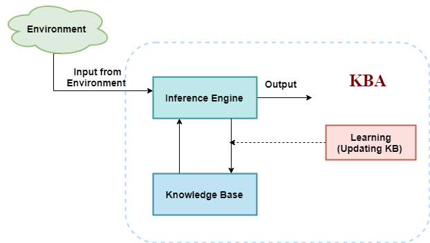
The above diagram is representing a generalized architecture for a knowledge-based agent. The knowledge-based agent (KBA) take input from the environment by perceiving the environment. The input is taken by the inference engine of the agent and which also communicate with KB to decide as per the knowledge store in KB. The learning element of KBA regularly updates the KB by learning new knowledge.

Knowledge base: Knowledge-base is a central component of a knowledge-based agent, it is also known as KB. It is a collection of sentences (here 'sentence' is a technical term and it is not identical to sentence in English). These sentences are expressed in a language which is called a knowledge representation language. The Knowledge-base of KBA stores fact about the world.

Why use a knowledge base?

Knowledge-base is required for updating knowledge for an agent to learn with experiences and take action as per the knowledge.

Inference system

Inference means deriving new sentences from old. Inference system allows us to add a new sentence to the knowledge base. A sentence is a proposition about the world. Inference system applies logical rules to the KB to deduce new information.

Inference system generates new facts so that an agent can update the KB. An inference system works mainly in two rules which are given as:

• Forward chaining
• Backward chaining

Operations Performed by KBA

Following are three operations which are performed by KBA in order to show the intelligent behavior:

1. TELL: This operation tells the knowledge base what it perceives from the environment.
2. ASK: This operation asks the knowledge base what action it should perform.
3. Perform: It performs the selected action.

A generic knowledge-based agent:

Following is the structure outline of a generic knowledge-based agents program:

1. Function KB-AGENT(percept):  
2. Persistent: KB, a knowledge base   
3.          t, a counter, initially 0, indicating time   
4. TELL(KB, MAKE-PERCEPT-SENTENCE(percept, t))   
5. Action = ASK(KB, MAKE-ACTION-QUERY(t))   
6. TELL(KB, MAKE-ACTION-SENTENCE(action, t))  
7. t = t + 1  
8. Return action   

The knowledge-based agent takes percept as input and returns an action as output. The agent maintains the knowledge base, KB, and it initially has some background knowledge of the real world. It also has a counter to indicate the time for the whole process, and this counter is initialized with zero.

Each time when the function is called, it performs its three operations:

• Firstly it TELLs the KB what it perceives.
• Secondly, it asks KB what action it should take
• Third agent program TELLS the KB that which action was chosen.

The MAKE-PERCEPT-SENTENCE generates a sentence as setting that the agent perceived the given percept at the given time.

The MAKE-ACTION-QUERY generates a sentence to ask which action should be done at the current time.

MAKE-ACTION-SENTENCE generates a sentence which asserts that the chosen action was executed.

Various levels of knowledge-based agent:

A knowledge-based agent can be viewed at different levels which are given below:

1. Knowledge level

Knowledge level is the first level of knowledge-based agent, and in this level, we need to specify what the agent knows, and what the agent goals are. With these specifications, we can fix its behavior. For example, suppose an automated taxi agent needs to go from a station A to station B, and he knows the way from A to B, so this comes at the knowledge level.

2. Logical level:

At this level, we understand that how the knowledge representation of knowledge is stored. At this level, sentences are encoded into different logics. At the logical level, an encoding of knowledge into logical sentences occurs. At the logical level we can expect to the automated taxi agent to reach to the destination B.

3. Implementation level:

This is the physical representation of logic and knowledge. At the implementation level agent perform actions as per logical and knowledge level. At this level, an automated taxi agent actually implement his knowledge and logic so that he can reach to the destination.

Approaches to designing a knowledge-based agent:

There are mainly two approaches to build a knowledge-based agent:

1. 1. Declarative approach: We can create a knowledge-based agent by initializing with an empty knowledge base and telling the agent all the sentences with which we want to start with. This approach is called Declarative approach.
2. 2. Procedural approach: In the procedural approach, we directly encode desired behavior as a program code. Which means we just need to write a program that already encodes the desired behavior or agent.

However, in the real world, a successful agent can be built by combining both declarative and procedural approaches, and declarative knowledge can often be compiled into more efficient procedural code.

2.2 Propositional logic

Propositional logic (PL) is the simplest form of logic where all the statements are made by propositions. A proposition is a declarative statement which is either true or false. It is a technique of knowledge representation in logical and mathematical form.

Example:

1. a) It is Sunday.  
2. b) The Sun rises from West (False proposition)  
3. c) 3+3= 7(False proposition)  
4. d) 5 is a prime number.   

Following are some basic facts about propositional logic:

• Propositional logic is also called Boolean logic as it works on 0 and 1.
• In propositional logic, we use symbolic variables to represent the logic, and we can use any symbol for a representing a proposition, such A, B, C, P, Q, R, etc.
• Propositions can be either true or false, but it cannot be both.
• Propositional logic consists of an object, relations or function, and logical connectives.
• These connectives are also called logical operators.
• The propositions and connectives are the basic elements of the propositional logic.
• Connectives can be said as a logical operator which connects two sentences.
• A proposition formula which is always true is called tautology, and it is also called a valid sentence.
• A proposition formula which is always false is called Contradiction.
• A proposition formula which has both true and false values is called
• Statements which are questions, commands, or opinions are not propositions such as "Where is Rohini", "How are you", "What is your name", are not propositions.

Syntax of propositional logic:

The syntax of propositional logic defines the allowable sentences for the knowledge representation. There are two types of Propositions:

1. Atomic Propositions
2. Compound propositions

• Atomic Proposition: Atomic propositions are the simple propositions. It consists of a single proposition symbol. These are the sentences which must be either true or false.

Example:

1. a) 2+2 is 4, it is an atomic proposition as it is a true fact.  
2. b) "The Sun is cold" is also a proposition as it is a false fact.   

• Compound proposition: Compound propositions are constructed by combining simpler or atomic propositions, using parenthesis and logical connectives.

Example:

1. a) "It is raining today, and street is wet."  
2. b) "Ankit is a doctor, and his clinic is in Mumbai."   

Logical Connectives:

Logical connectives are used to connect two simpler propositions or representing a sentence logically. We can create compound propositions with the help of logical connectives. There are mainly five connectives, which are given as follows:

1. Negation: A sentence such as ¬ P is called negation of P. A literal can be either Positive literal or negative literal.
2. Conjunction: A sentence which has ∧ connective such as, P ∧ Q is called a conjunction.
   Example: Rohan is intelligent and hardworking. It can be written as,
   P= Rohan is intelligent,
   Q= Rohan is hardworking. → P∧ Q.
3. Disjunction: A sentence which has ∨ connective, such as P ∨ Q. Is called disjunction, where P and Q are the propositions.
   Example: "Ritika is a doctor or Engineer",
   Here P= Ritika is Doctor. Q= Ritika is Doctor, so we can write it as P ∨ Q.
4. Implication: A sentence such as P → Q, is called an implication. Implications are also known as if-then rules. It can be represented as
               If it is raining, then the street is wet.
           Let P= It is raining, and Q= Street is wet, so it is represented as P → Q
5. Biconditional: A sentence such as P⇔ Q is a Biconditional sentence, example If I am breathing, then I am alive
               P= I am breathing, Q= I am alive, it can be represented as P ⇔ Q.

Following is the summarized table for Propositional Logic Connectives:

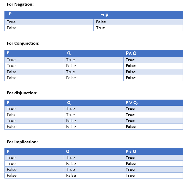
Truth Table:

In propositional logic, we need to know the truth values of propositions in all possible scenarios. We can combine all the possible combination with logical connectives, and the representation of these combinations in a tabular format is called Truth table. Following are the truth table for all logical connectives:

Truth table with three propositions:

We can build a proposition composing three propositions P, Q, and R. This truth table is made-up of 8n Tuples as we have taken three proposition symbols.

Precedence of connectives:

Just like arithmetic operators, there is a precedence order for propositional connectors or logical operators. This order should be followed while evaluating a propositional problem. Following is the list of the precedence order for operators:

Note: For better understanding use parenthesis to make sure of the correct interpretations. Such as ¬R∨ Q, It can be interpreted as (¬R) ∨ Q.

Logical equivalence:

Logical equivalence is one of the features of propositional logic. Two propositions are said to be logically equivalent if and only if the columns in the truth table are identical to each other.

Let's take two propositions A and B, so for logical equivalence, we can write it as A⇔B. In below truth table we can see that column for ¬A∨ B and A→B, are identical hence A is Equivalent to B

Properties of Operators:

• Commutativity:
  • P∧ Q= Q ∧ P, or
  • P ∨ Q = Q ∨ P.
• Associativity:
  • (P ∧ Q) ∧ R= P ∧ (Q ∧ R),
  • (P ∨ Q) ∨ R= P ∨ (Q ∨ R)
• Identity element:
  • P ∧ True = P,
  • P ∨ True= True.
• Distributive:
  • P∧ (Q ∨ R) = (P ∧ Q) ∨ (P ∧ R).
  • P ∨ (Q ∧ R) = (P ∨ Q) ∧ (P ∨ R).
• DE Morgan's Law:
  • ¬ (P ∧ Q) = (¬P) ∨ (¬Q)
  • ¬ (P ∨ Q) = (¬ P) ∧ (¬Q).
• Double-negation elimination:
  • ¬ (¬P) = P.

Limitations of Propositional logic:

• We cannot represent relations like ALL, some, or none with propositional logic. Example:
  1. All the girls are intelligent.
  2. Some apples are sweet.
• Propositional logic has limited expressive power.
• In propositional logic, we cannot describe statements in terms of their properties or logical relationships.

2.3 First order logic

In the topic of Propositional logic, we have seen that how to represent statements using propositional logic. But unfortunately, in propositional logic, we can only represent the facts, which are either true or false. PL is not sufficient to represent the complex sentences or natural language statements. The propositional logic has very limited expressive power. Consider the following sentence, which we cannot represent using PL logic.

• "Some humans are intelligent", or
• "Sachin likes cricket."

To represent the above statements, PL logic is not sufficient, so we required some more powerful logic, such as first-order logic.

First-Order logic:

• First-order logic is another way of knowledge representation in artificial intelligence. It is an extension to propositional logic.
• FOL is sufficiently expressive to represent the natural language statements in a concise way.
• First-order logic is also known as Predicate logic or First-order predicate logic. First-order logic is a powerful language that develops information about the objects in a more easy way and can also express the relationship between those objects.
• First-order logic (like natural language) does not only assume that the world contains facts like propositional logic but also assumes the following things in the world:
  • Objects: A, B, people, numbers, colors, wars, theories, squares, pits, wumpus, ......
  • Relations: It can be unary relation such as: red, round, is adjacent, or n-any relation such as: the sister of, brother of, has color, comes between
  • Function: Father of, best friend, third inning of, end of, ......
• As a natural language, first-order logic also has two main parts:
  1. Syntax
  2. Semantics

Syntax of First-Order logic:

The syntax of FOL determines which collection of symbols is a logical expression in first-order logic. The basic syntactic elements of first-order logic are symbols. We write statements in short-hand notation in FOL.

Basic Elements of First-order logic:

Following are the basic elements of FOL syntax:

Atomic sentences:

• Atomic sentences are the most basic sentences of first-order logic. These sentences are formed from a predicate symbol followed by a parenthesis with a sequence of terms.
• We can represent atomic sentences as Predicate (term1, term2, ......, term n).

Example: Ravi and Ajay are brothers: => Brothers(Ravi, Ajay).
                Chinky is a cat: => cat (Chinky).

Complex Sentences:

• Complex sentences are made by combining atomic sentences using connectives.

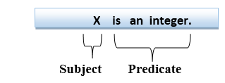
First-order logic statements can be divided into two parts:

• Subject: Subject is the main part of the statement.
• Predicate: A predicate can be defined as a relation, which binds two atoms together in a statement.

Consider the statement: "x is an integer.", it consists of two parts, the first part x is the subject of the statement and second part "is an integer," is known as a predicate.

Quantifiers in First-order logic:

• A quantifier is a language element which generates quantification, and quantification specifies the quantity of specimen in the universe of discourse.
• These are the symbols that permit to determine or identify the range and scope of the variable in the logical expression. There are two types of quantifier:
  1. Universal Quantifier, (for all, everyone, everything)
  2. Existential quantifier, (for some, at least one).

Universal Quantifier:

Universal quantifier is a symbol of logical representation, which specifies that the statement within its range is true for everything or every instance of a particular thing.

The Universal quantifier is represented by a symbol ∀, which resembles an inverted A.

Note: In universal quantifier we use implication "→".

If x is a variable, then ∀x is read as:

• For all x
• For each x
• For every x.

Example:

All man drink coffee.

Let a variable x which refers to a cat so all x can be represented in UOD as below:

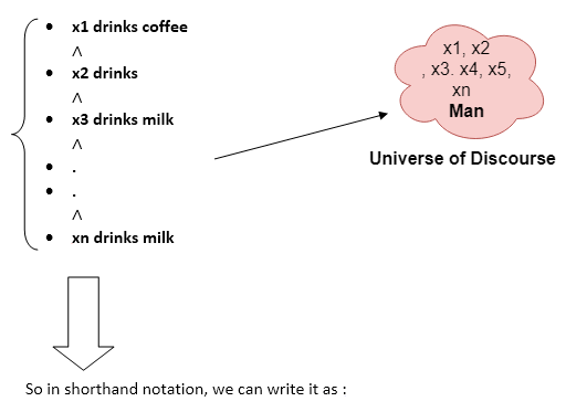
∀x man(x) → drink (x, coffee).

It will be read as: There are all x where x is a man who drink coffee.

Existential Quantifier:

Existential quantifiers are the type of quantifiers, which express that the statement within its scope is true for at least one instance of something.

It is denoted by the logical operator ∃, which resembles as inverted E. When it is used with a predicate variable then it is called as an existential quantifier.

Note: In Existential quantifier we always use AND or Conjunction symbol (∧).

If x is a variable, then existential quantifier will be ∃x or ∃(x). And it will be read as:

• There exists a 'x.'
• For some 'x.'
• For at least one 'x.'

Example:

Some boys are intelligent.

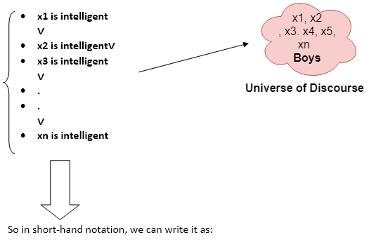
∃x: boys(x) ∧ intelligent(x)

It will be read as: There are some x where x is a boy who is intelligent.

Points to remember:

• The main connective for universal quantifier ∀ is implication →.
• The main connective for existential quantifier ∃ is and ∧.

Properties of Quantifiers:

• In universal quantifier, ∀x∀y is similar to ∀y∀x.
• In Existential quantifier, ∃x∃y is similar to ∃y∃x.
• ∃x∀y is not similar to ∀y∃x.

Some Examples of FOL using quantifier:

1. All birds fly.
In this question the predicate is "fly(bird)."
And since there are all birds who fly so it will be represented as follows.
              ∀x bird(x) →fly(x).

2. Every man respects his parent.
In this question, the predicate is "respect(x, y)," where x=man, and y= parent.
Since there is every man so will use ∀, and it will be represented as follows:
              ∀x man(x) → respects (x, parent).

3. Some boys play cricket.
In this question, the predicate is "play(x, y)," where x= boys, and y= game. Since there are some boys so we will use ∃, and it will be represented as:
              ∃x boys(x) → play(x, cricket).

4. Not all students like both Mathematics and Science.
In this question, the predicate is "like(x, y)," where x= student, and y= subject.
Since there are not all students, so we will use ∀ with negation, so following representation for this:
              ¬∀ (x) [ student(x) → like(x, Mathematics) ∧ like(x, Science)].

5. Only one student failed in Mathematics.
In this question, the predicate is "failed(x, y)," where x= student, and y= subject.
Since there is only one student who failed in Mathematics, so we will use following representation for this:
              ∃(x) [ student(x) → failed (x, Mathematics) ∧∀ (y) [¬(x==y) ∧ student(y) → ¬failed (x, Mathematics)].

Free and Bound Variables:

The quantifiers interact with variables which appear in a suitable way. There are two types of variables in First-order logic which are given below:

Free Variable: A variable is said to be a free variable in a formula if it occurs outside the scope of the quantifier.

Example: ∀x ∃(y)[P (x, y, z)], where z is a free variable.

Bound Variable: A variable is said to be a bound variable in a formula if it occurs within the scope of the quantifier.

Example: ∀x [A (x) B( y)], here x and y are the bound variables.

2.4 Inference in first order logic

Inference in First-Order Logic is used to deduce new facts or sentences from existing sentences. Before understanding the FOL inference rule, let's understand some basic terminologies used in FOL.

Substitution:

Substitution is a fundamental operation performed on terms and formulas. It occurs in all inference systems in first-order logic. The substitution is complex in the presence of quantifiers in FOL. If we write F[a/x], so it refers to substitute a constant "a" in place of variable "x".

Note: First-order logic is capable of expressing facts about some or all objects in the universe.

Equality:

First-Order logic does not only use predicate and terms for making atomic sentences but also uses another way, which is equality in FOL. For this, we can use equality symbols which specify that the two terms refer to the same object.

Example: Brother (John) = Smith.

As in the above example, the object referred by the Brother (John) is similar to the object referred by Smith. The equality symbol can also be used with negation to represent that two terms are not the same objects.

Example: ￢(x=y) which is equivalent to x ≠y.

FOL inference rules for quantifier:

As propositional logic we also have inference rules in first-order logic, so following are some basic inference rules in FOL:

• Universal Generalization
• Universal Instantiation
• Existential Instantiation
• Existential introduction

1. Universal Generalization:

• Universal generalization is a valid inference rule which states that if premise P(c) is true for any arbitrary element c in the universe of discourse, then we can have a conclusion as ∀ x P(x).
• It can be represented as: .
• This rule can be used if we want to show that every element has a similar property.
• In this rule, x must not appear as a free variable.

Example: Let's represent, P(c): "A byte contains 8 bits", so for ∀ x P(x) "All bytes contain 8 bits.", it will also be true.

2. Universal Instantiation:

• Universal instantiation is also called as universal elimination or UI is a valid inference rule. It can be applied multiple times to add new sentences.
• The new KB is logically equivalent to the previous KB.
• As per UI, we can infer any sentence obtained by substituting a ground term for the variable.
• The UI rule state that we can infer any sentence P(c) by substituting a ground term c (a constant within domain x) from ∀ x P(x) for any object in the universe of discourse.
• It can be represented as:.

Example:1.

IF "Every person like ice-cream"=> ∀x P(x) so we can infer that
"John likes ice-cream" => P(c)

Example: 2.

Let's take a famous example,

"All kings who are greedy are Evil." So let our knowledge base contains this detail as in the form of FOL:

∀x king(x) ∧ greedy (x) → Evil (x),

So from this information, we can infer any of the following statements using Universal Instantiation:

• King(John) ∧ Greedy (John) → Evil (John),
• King(Richard) ∧ Greedy (Richard) → Evil (Richard),
• King(Father(John)) ∧ Greedy (Father(John)) → Evil (Father(John)),

3. Existential Instantiation:

• Existential instantiation is also called as Existential Elimination, which is a valid inference rule in first-order logic.
• It can be applied only once to replace the existential sentence.
• The new KB is not logically equivalent to old KB, but it will be satisfiable if old KB was satisfiable.
• This rule states that one can infer P(c) from the formula given in the form of ∃x P(x) for a new constant symbol c.
• The restriction with this rule is that c used in the rule must be a new term for which P(c ) is true.
• It can be represented as:

Example:

From the given sentence: ∃x Crown(x) ∧ OnHead(x, John),

So we can infer: Crown(K) ∧ OnHead( K, John), as long as K does not appear in the knowledge base.

• The above used K is a constant symbol, which is called Skolem constant.
• The Existential instantiation is a special case of Skolemization process.

4. Existential introduction

• An existential introduction is also known as an existential generalization, which is a valid inference rule in first-order logic.
• This rule states that if there is some element c in the universe of discourse which has a property P, then we can infer that there exists something in the universe which has the property P.
• It can be represented as:
• Example: Let's say that,
  "Priyanka got good marks in English."
  "Therefore, someone got good marks in English."

Generalized Modus Ponens Rule:

For the inference process in FOL, we have a single inference rule which is called Generalized Modus Ponens. It is lifted version of Modus ponens.

Generalized Modus Ponens can be summarized as, " P implies Q and P is asserted to be true, therefore Q must be True."

According to Modus Ponens, for atomic sentences pi, pi', q. Where there is a substitution θ such that SUBST (θ, pi',) = SUBST(θ, pi), it can be represented as:

Example:

We will use this rule for Kings are evil, so we will find some x such that x is king, and x is greedy so we can infer that x is evil.

1. Here let say, p1' is king(John)        p1 is king(x)  
2. p2' is Greedy(y)                       p2 is Greedy(x)  
3. θ is {x/John, y/John}                  q is evil(x)  
4. SUBST(θ,q).                                                        

2.5 Resolution – refutation proofs

Resolution

Resolution is a theorem proving technique that proceeds by building refutation proofs, i.e., proofs by contradictions. It was invented by a Mathematician John Alan Robinson in the year 1965.

Resolution is used, if there are various statements are given, and we need to prove a conclusion of those statements. Unification is a key concept in proofs by resolutions. Resolution is a single inference rule which can efficiently operate on the conjunctive normal form or clausal form.

Clause: Disjunction of literals (an atomic sentence) is called a clause. It is also known as a unit clause.

Conjunctive Normal Form: A sentence represented as a conjunction of clauses is said to be conjunctive normal form or CNF.

Note: To better understand this topic, firstly learns the FOL in AI.

The resolution inference rule:

The resolution rule for first-order logic is simply a lifted version of the propositional rule. Resolution can resolve two clauses if they contain complementary literals, which are assumed to be standardized apart so that they share no variables.

Where li and mj are complementary literals.

This rule is also called the binary resolution rule because it only resolves exactly two literals.

Example:

We can resolve two clauses which are given below:

[Animal (g(x) V Loves (f(x), x)]       and       [￢ Loves(a, b) V ￢Kills(a, b)]

Where two complimentary literals are: Loves (f(x), x) and ￢ Loves (a, b)

These literals can be unified with unifier θ= [a/f(x), and b/x] , and it will generate a resolvent clause:

[Animal (g(x) V ￢ Kills(f(x), x)].

Steps for Resolution:

1. Conversion of facts into first-order logic.
2. Convert FOL statements into CNF
3. Negate the statement which needs to prove (proof by contradiction)
4. Draw resolution graph (unification).

To better understand all the above steps, we will take an example in which we will apply resolution.

Example:

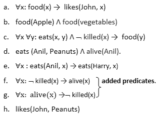
1. John likes all kind of food.
2. Apple and vegetable are food
3. Anything anyone eats and not killed is food.
4. Anil eats peanuts and still alive
5. Harry eats everything that Anil eats.
   Prove by resolution that:
6. John likes peanuts.

Step-1: Conversion of Facts into FOL

In the first step we will convert all the given statements into its first order logic.

Step-2: Conversion of FOL into CNF

In First order logic resolution, it is required to convert the FOL into CNF as CNF form makes easier for resolution proofs.

• Eliminate all implication (→) and rewrite
  1. ∀x ¬ food(x) V likes(John, x)
  2. Food(Apple) Λ food(vegetables)
  3. ∀x ∀y ¬ [eats(x, y) Λ ¬ killed(x)] V food(y)
  4. Eats (Anil, Peanuts) Λ alive(Anil)
  5. ∀x ¬ eats(Anil, x) V eats(Harry, x)
  6. ∀x¬ [¬ killed(x) ] V alive(x)
  7. ∀x ¬ alive(x) V ¬ killed(x)
  8. Likes(John, Peanuts).
• Move negation (¬)inwards and rewrite
  1. ∀x ¬ food(x) V likes(John, x)
  2. Food(Apple) Λ food(vegetables)
  3. ∀x ∀y ¬ eats(x, y) V killed(x) V food(y)
  4. Eats (Anil, Peanuts) Λ alive(Anil)
  5. ∀x ¬ eats(Anil, x) V eats(Harry, x)
  6. ∀x ¬killed(x) ] V alive(x)
  7. ∀x ¬ alive(x) V ¬ killed(x)
  8. Likes(John, Peanuts).
• Rename variables or standardize variables
  1. ∀x ¬ food(x) V likes(John, x)
  2. Food(Apple) Λ food(vegetables)
  3. ∀y ∀z ¬ eats(y, z) V killed(y) V food(z)
  4. Eats (Anil, Peanuts) Λ alive(Anil)
  5. ∀w¬ eats(Anil, w) V eats(Harry, w)
  6. ∀g ¬killed(g) ] V alive(g)
  7. ∀k ¬ alive(k) V ¬ killed(k)
  8. Likes(John, Peanuts).
• Eliminate existential instantiation quantifier by elimination.
  In this step, we will eliminate existential quantifier ∃, and this process is known as Skolemization. But in this example problem since there is no existential quantifier so all the statements will remain same in this step.
• Drop Universal quantifiers.
  In this step we will drop all universal quantifier since all the statements are not implicitly quantified so we don't need it.
  1. ¬ food(x) V likes(John, x)
  2. Food(Apple)
  3. Food(vegetables)
  4. ¬ eats(y, z) V killed(y) V food(z)
  5. Eats (Anil, Peanuts)
  6. Alive(Anil)
  7. ¬ eats(Anil, w) V eats(Harry, w)
  8. Killed(g) V alive(g)
  9. ¬ alive(k) V ¬ killed(k)
  10. Likes(John, Peanuts).

Note: Statements "food(Apple) Λ food(vegetables)" and "eats (Anil, Peanuts) Λ alive(Anil)" can be written in two separate statements.

• Distribute conjunction ∧ over disjunction ¬.
  This step will not make any change in this problem.

Step-3: Negate the statement to be proved

In this statement, we will apply negation to the conclusion statements, which will be written as ¬likes(John, Peanuts)

Step-4: Draw Resolution graph:

Now in this step, we will solve the problem by resolution tree using substitution. For the above problem, it will be given as follows:

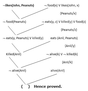
Hence the negation of the conclusion has been proved as a complete contradiction with the given set of statements.

Explanation of Resolution graph:

• In the first step of resolution graph, ¬likes(John, Peanuts) , and likes(John, x) get resolved(canceled) by substitution of {Peanuts/x}, and we are left with ¬ food(Peanuts)
• In the second step of the resolution graph, ¬ food(Peanuts) , and food(z) get resolved (canceled) by substitution of { Peanuts/z}, and we are left with ¬ eats(y, Peanuts) V killed(y) .
• In the third step of the resolution graph, ¬ eats(y, Peanuts) and eats (Anil, Peanuts) get resolved by substitution {Anil/y}, and we are left with Killed(Anil) .
• In the fourth step of the resolution graph, Killed(Anil) and ¬ killed(k) get resolve by substitution {Anil/k}, and we are left with ¬ alive(Anil) .
• In the last step of the resolution graph ¬ alive(Anil) and alive(Anil) get resolved.

2.6 Theorem Proving in First Order Logic

Why theorem proving in an AI course?

• Proving theorems is considered to require high intelligence
• If knowledge is represented by logic, theorem proving is reasoning
• Theorem proving uses AI techniques, such as (heuristic) search
• (study how people prove theorems. Differently!)

What is theorem proving?

Reasoning by theorem proving is a weak method, compared to experts systems, because it does not make use of domain knowledge. This, on the other hand, may be a strength, if no domain heuristics are available (reasoning from first principles). Theorem proving is usually limited to sound reasoning.

Differentiate between

• Theorem provers: fully automatic
• Proof assistants: require steps as input, take care of bookkeeping and sometimes 'easy' proofs.

Theorem proving requires

• a logic (syntax)
• a set of axioms and inference rules
• a strategy on when how to search through the possible applications of the axioms and rules

Examples of axioms
p -> (q->p)
(p->(q->r)) -> ((p->q) ->(p->r))
p \/ ~p
p->(~p->q)
Notation: I use ~ for "not", since it's on my keyboard.

Examples of inference rules
 

Strategies
forwards - start from axioms, apply rules
backwards - start from the theorem (in general: a set of goals), work backwards to the axioms

Depth-first or breadth-first

When to apply which rule

General questions:
are the rules correct (sound)?
is there a proof for every logical consequence (complete)?
can we remove rules (redundant)?
Having redundant rules may allow shorter proofs, but a larger search space.

Resolution and refutation

We want to prove theory -> goal.
The theory is usually a set of facts and rules, that can be treated as axioms (by the rule called implication above). A theory is usually quite stable, and used to prove various goals.

• We use contradiction, add ~goal to the axioms, and try to prove false.
• The theory and ~goal are put in clausal form - a set (conjunction) of  clauses
  [see Luger p 558-560]
• Use resolution and unification to derive false

Clauses
a clause is a universially quantified disjunction of literals
a literal is an atomic formula or its negation
examples of clauses: p \/ q, p(X) \/ q(Y), ~p(X) \/ q(X).
A special case is Horn-clauses: they have at most one positive (not negated) literal.
Three subclasses:
facts (1 pos, 0 neg): p(a,b).
rules (1 pos, > 0 neg): ~p \/ ~q \/ r - often written as: p /\ q -> r
goals(0 pos): ~p \/ ~q - if we want to prove p/\q from the theory, we add this clause - can be written as p /\ q -> false

Skolemization (p. 559)
How to remove existential quantification? Use function symbols!
Example: every person has a mother: (for all X) person(X) -> (exists Y) mother(X,Y)
Give a name to Y: the mother of X. (for all X) person(X) -> mother(X,mother_of(X))

This allows us to define datastructures in the logic.
Example: if X is an element and Y a list, then there is a list with head X and tail Y.
(for all X,Y) elt(X) /\ list(Y) -> (exists Z) list(Z) /\ head(Z,X) /\ tail(Z,Y)
first we name Z the cons of X and Y, then we get 3 rules:
elt(X) /\ list(Y) -> list(cons(X,Y)).
elt(X) /\ list(Y) -> head(cons(X,Y), X).
elt(X) /\ list(Y) -> tail(cons(X,Y), Y).

Unification

Unification (2.3.2) is used to perform instantiation before (during) resolution.

Simple case:
Resolve list(nil) with ~elt(X) \/ ~list(Y) \/ list(cons(X,Y)).
First we must instantiate Y to nil, then we can derive ~elt(X) \/ list(cons(X,nil)).

Hard case:
I want to prove that there is a list that has the head mother_of(john).
So I take as a goal its negation ~(exists X)(list(X) /\ head(X,mother_of(john)))
This gives the clause  ~list(X) \/ ~head(X,mother_of(john))
We can resolve with ~elt(X) \/ ~list(Y) \/ head(cons(X,Y),X).
Problem 1: the X's in both clauses "accidentally" have the same name.
Solution 1: rename to ~elt(Z) \/ ~list(Y) \/ head(cons(Z,Y),Z).
Problem 2: what is the common instance of head(cons(Z,Y),Z) and head(X,mother_of(john))?
Answer - the result of unification: head(cons(mother_of(john),Y),mother_of(john))
The unifier is: {Z/mother_of(john), X/cons(mother_of(john),Y)}
The resolvent (resulting clause) is
(~list(X) \/ ~elt(Z) \/ ~list(Y)){Z/mother_of(john), X/cons(mother_of(john),Y)} =
~list(cons(mother_of(john),Y)) \/ ~elt(mother_of(john)) \/ ~list(Y)

Exercise: use the first list-rule and the facts elt(mother_of(john)) and list(nil)to complete the proof.

Unification as rewriting
the algorithm maintains a set of equalities. Each time, remove an equality and apply the applicable  rule.

• Var1 = Var1 - nothing (just remove the equality)
• Var1 = Expr - in all other equalities, replace Var1 by Expr, keep Var1 = Expr
  exception: if Var1 occurs in Expr, then FAIL
• f(A1,..,An) = f(B1,..,Bn) - add {A1 = B1, .., An = Bn}
• f(A1,..,An) = g(B1,..,Bm) - FAIL

Example (the equality selected is underlined)
{head(cons(Z,Y),Z) = head(X,mother_of(john))} - use the first f-rule, f=head, n=2.
{cons(Z,Y) = X, Z = mother_of(john)}
{cons(mother_of(john),Y) = X, Z = mother_of(john)}
no more applicable rules, and no FAIL, so we have a unifier.

Resolution and Prolog

A Prolog program consists of Horn-clauses: facts and rules.
We give the program a goal, which it turns into a Horn clause with only negative literals.
Prolog uses linear resolution:
it takes the goal and a rule/fact, and produces a new goal, until it derives false. This proves the goal.
(Other outcomes are that Prolog runs out of options and cannot prove the goal, or that it goes into an infinite loop.)
Linear resolution is not complete for predicate logic in general, but it is complete in this special case.
Prolog uses depth-first search in a search tree - choices arise when more than one rule is applicable.

2.7 Planning

What is planning in AI?

• The planning in Artificial Intelligence is about the decision making tasks performed by the robots or computer programs to achieve a specific goal.
• The execution of planning is about choosing a sequence of actions with a high likelihood to complete the specific task.

Blocks-World planning problem

• The blocks-world problem is known as Sussman Anomaly.
• Noninterleaved planners of the early 1970s were unable to solve this problem, hence it is considered as anomalous.
• When two subgoals G1 and G2 are given, a noninterleaved planner produces either a plan for G1 concatenated with a plan for G2, or vice-versa.
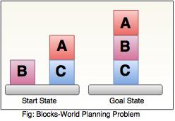
• In blocks-world problem, three blocks labeled as 'A', 'B', 'C' are allowed to rest on the flat surface. The given condition is that only one block can be moved at a time to achieve the goal.
• The start state and goal state are shown in the following diagram.

Components of Planning System

The planning consists of following important steps:

• Choose the best rule for applying the next rule based on the best available heuristics.
• Apply the chosen rule for computing the new problem state.
• Detect when a solution has been found.
• Detect dead ends so that they can be abandoned and the system’s effort is directed in more fruitful directions.
• Detect when an almost correct solution has been found.

Goal stack planning

This is one of the most important planning algorithms, which is specifically used by STRIPS.

• The stack is used in an algorithm to hold the action and satisfy the goal.  A knowledge base is used to hold the current state, actions.
• Goal stack is similar to a node in a search tree, where the branches are created if there is a choice of an action.

The important steps of the algorithm are as stated below:

i. Start by pushing the original goal on the stack. Repeat this  until the stack becomes empty. If stack top is a compound goal, then push its unsatisfied subgoals on the stack.
ii. If stack top is a single unsatisfied goal then, replace it by an action and push the action’s precondition on the stack to satisfy the condition.
iii. If stack top is an action, pop it from the stack, execute it and change the knowledge base by the effects of the action.
iv. If stack top is a satisfied goal, pop it from the stack.

Non-linear planning

This planning is used to set a goal stack and is included in the search space of all possible subgoal orderings. It handles the goal interactions by interleaving method.

Advantage of non-Linear planning
Non-linear planning may be an optimal solution with respect to plan length (depending on search strategy used).

Disadvantages of Nonlinear planning

• It takes larger search space, since all possible goal orderings are taken into consideration.
• Complex algorithm to understand.

Algorithm
1. Choose a goal 'g' from the goalset
2. If 'g' does not match the state, then

• Choose an operator 'o' whose add-list matches goal g
• Push 'o' on the opstack
• Add the preconditions of 'o' to the goalset

3. While all preconditions of operator on top of opstack are met in state

• Pop operator o from top of opstack
• State = apply(o, state)
• Plan = [plan; o]

2.8 Partial order planning

The forward and regression planners enforce a total ordering on actions at all stages of the planning process. The CSP planner commits to the particular time that the action will be carried out. This means that those planners have to commit to an ordering of actions that cannot occur concurrently when adding them to a partial plan, even if there is no particular reason to put one action before another.

The idea of a partial-order planner is to have a partial ordering between actions and only commit to an ordering between actions when forced. This is sometimes also called a non-linear planner, which is a misnomer because such planners often produce a linear plan.

A partial ordering is a less-than relation that is transitive and asymmetric. A partial-order plan is a set of actions together with a partial ordering, representing a "before" relation on actions, such that any total ordering of the actions, consistent with the partial ordering, will solve the goal from the initial state. Write act0 < act1 if action act0 is before action act1 in the partial order. This means that action act0 must occur before action act1.

For uniformity, treat start as an action that achieves the relations that are true in the initial state, and treat finish as an action whose precondition is the goal to be solved. The pseudoaction start is before every other action, and finish is after every other action. The use of these as actions means that the algorithm does not require special cases for the initial situation and for the goals. When the preconditions of finish hold, the goal is solved.

An action, other than start or finish, will be in a partial-order plan to achieve a precondition of an action in the plan. Each precondition of an action in the plan is either true in the initial state, and so achieved by start, or there will be an action in the plan that achieves it.

We must ensure that the actions achieve the conditions they were assigned to achieve. Each precondition P of an action act1 in a plan will have an action act0 associated with it such that act0 achieves precondition P for act1. The triple ⟨act0,P,act1⟩ is a causal link. The partial order specifies that action act0 occurs before action act1, which is written as act0 < act1. Any other action A that makes P false must either be before act0 or after act1.

Informally, a partial-order planner works as follows: Begin with the actions start and finish and the partial order start < finish. The planner maintains an agenda that is a set of ⟨P,A⟩ pairs, where A is an action in the plan and P is an atom that is a precondition of A that must be achieved. Initially the agenda contains pairs ⟨G,finish⟩, where G is an atom that must be true in the goal state.

At each stage in the planning process, a pair ⟨G,act1⟩ is selected from the agenda, where P is a precondition for action act1. Then an action, act0, is chosen to achieve P. That action is either already in the plan - it could be the start action, for example - or it is a new action that is added to the plan. Action act0 must happen before act1 in the partial order. It adds a causal link that records that act0 achieves P for action act1. Any action in the plan that deletes P must happen either before act0 or after act1. If act0 is a new action, its preconditions are added to the agenda, and the process continues until the agenda is empty.

This is a non-deterministic procedure. The "choose" and the "either ...or ..." form choices that must be searched over. There are two choices that require search:

• Which action is selected to achieve G and
• Whether an action that deletes G happens before act0 or after act1.

Non-deterministic procedure PartialOrderPlanner(Gs)
2:           Inputs
3:                     Gs: set of atomic propositions to achieve
4:           Output
5:                     linear plan to achieve Gs
6:           Local
7:                     Agenda: set of ⟨P,A⟩ pairs where P is atom and A an action
8:                     Actions: set of actions in the current plan
9:                     Constraints: set of temporal constraints on actions
10:                     CausalLinks: set of ⟨act0,P,act1⟩ triples
11:           Agenda ←{⟨G,finish⟩:G ∈Gs}
12:           Actions ←{start,finish}
13:           Constraints ←{start<finish}
14:           CausalLinks ←{}
15:           repeat
16:                     select and remove ⟨G,act1⟩ from Agenda
17:                     either
18:                               choose act0 ∈Actions such that act0 achieves G
19:                     or
20:                               choose act0 ∉Actions such that act0 achieves G
21:                               Actions ←Actions ∪{act0}
22:                               Constraints ←add_const(start<act0,Constraints)
23:                               for each CL∈CausalLinks do
24:                                         Constraints ←protect(CL,act0,Constraints)
25:                               
26:                               Agenda ←Agenda ∪{⟨P,act0⟩: P is a precondition of act0 }
27:                     
28 :                    Constraints ←add_const(act0<act1,Constraints)
29:                     CausalLinks ∪ {⟨acto,G,act1⟩}
30:                     for each A∈Actions do
31:                               Constraints ←protect(⟨acto,G,act1⟩,A,Constraints)
32:                               
33:           until Agenda={}
34:           return total ordering of Actions consistent with Constraints

Figure 8.5: Partial-order planner

The function add_const(act0<act1,Constraints) returns the constraints formed by adding the constraint act0<act1 to Constraints, and it fails if act0<act1 is incompatible with Constraints. There are many ways this function can be implemented.

The function protect(⟨acto,G,act1⟩,A,Constraints) checks whether A≠act0 and A≠act1 and A deletes G. If so, it returns either { A<act0 } ∪ Constraints or { act1<A } ∪ Constraints. This is a non-deterministic choice that is searched over. Otherwise it returns Constraints.

Example 8.14: Consider the goal ¬swc ∧ ¬mw, where the initial state contains RLoc=lab, swc, ¬rhc, mw, ¬rhm.

Initially the agenda is

⟨ ¬swc,finish⟩,⟨ ¬mw,finish⟩.

Suppose ⟨ ¬swc,finish⟩ is selected and removed from the agenda. One action exists that can achieve ¬swc, namely deliver coffee, dc, with preconditions off and rhc. At the end of the repeat loop, Agenda contains

⟨off,dc⟩,⟨rhc,dc⟩,⟨ ¬mw,finish⟩.

Constraints is {start<finish, start < dc, dc <finish}. There is one causal link, ⟨dc, ¬swc,finish⟩. This causal link means that no action that undoes ¬swc is allowed to happen after dc and before finish.

Suppose ⟨ ¬mw,finish⟩ is selected from the agenda. One action exists that can achieve this, pum, with preconditions mw and RLoc=mr. The causal link ⟨pum, ¬mw,finish⟩ is added to the set of causal links; ⟨mw,pum⟩ and ⟨mr,pum⟩ are added to the agenda.

Suppose ⟨mw,pum⟩ is selected from the agenda. The action start achieves mw, because mw is true initially. The causal link ⟨start,mw,pum⟩ is added to the set of causal links. Nothing is added to the agenda.

At this stage, there is no ordering imposed between dc and pum.

Suppose ⟨off,dc⟩ is removed from the agenda. There are two actions that can achieve off: mc_cs with preconditions cs, and mcc_lab with preconditions lab. The algorithm searches over these choices. Suppose it chooses mc_cs. Then the causal link ⟨mc_cs,off,dc⟩ is added.

The first violation of a causal link occurs when a move action is used to achieve ⟨mr,pum⟩. This action violates the causal link ⟨mc_cs,off,dc⟩, and so must happen after dc (the robot goes to the mail room after delivering coffee) or before mc_cs.

The preceding algorithm has glossed over one important detail. It is sometimes necessary to perform some action more than once in a plan. The preceding algorithm will not work in this case, because it will try to find a partial ordering with both instances of the action occurring at the same time. To fix this problem, the ordering should be between action instances, and not actions themselves. To implement this, assign an index to each instance of an action in the plan, and the ordering is on the action instance indexes and not the actions themselves. This is left as an exercise.

2.9 Uncertain Knowledge and Reasoning

Uncertainty:

Till now, we have learned knowledge representation using first-order logic and propositional logic with certainty, which means we were sure about the predicates. With this knowledge representation, we might write A→B, which means if A is true then B is true, but consider a situation where we are not sure about whether A is true or not then we cannot express this statement, this situation is called uncertainty.

So to represent uncertain knowledge, where we are not sure about the predicates, we need uncertain reasoning or probabilistic reasoning.

Causes of uncertainty:

Following are some leading causes of uncertainty to occur in the real world.

1. Information occurred from unreliable sources.
2. Experimental Errors
3. Equipment fault
4. Temperature variation
5. Climate change.

Probabilistic reasoning:

Probabilistic reasoning is a way of knowledge representation where we apply the concept of probability to indicate the uncertainty in knowledge. In probabilistic reasoning, we combine probability theory with logic to handle the uncertainty.

We use probability in probabilistic reasoning because it provides a way to handle the uncertainty that is the result of someone's laziness and ignorance.

In the real world, there are lots of scenarios, where the certainty of something is not confirmed, such as "It will rain today," "behavior of someone for some situations," "A match between two teams or two players." These are probable sentences for which we can assume that it will happen but not sure about it, so here we use probabilistic reasoning.

Need of probabilistic reasoning in AI:

• When there are unpredictable outcomes.
• When specifications or possibilities of predicates becomes too large to handle.
• When an unknown error occurs during an experiment.

In probabilistic reasoning, there are two ways to solve problems with uncertain knowledge:

• Bayes' rule
• Bayesian Statistics

Note: We will learn the above two rules in later chapters.

As probabilistic reasoning uses probability and related terms, so before understanding probabilistic reasoning, let's understand some common terms:

Probability: Probability can be defined as a chance that an uncertain event will occur. It is the numerical measure of the likelihood that an event will occur. The value of probability always remains between 0 and 1 that represent ideal uncertainties.

1. 0 ≤ P(A) ≤ 1,   where P(A) is the probability of an event A.  

1. P(A) = 0,  indicates total uncertainty in an event A.   

1. P(A) =1, indicates total certainty in an event A.    

We can find the probability of an uncertain event by using the below formula.

• P(¬A) = probability of a not happening event.
• P(¬A) + P(A) = 1.

Event: Each possible outcome of a variable is called an event.

Sample space: The collection of all possible events is called sample space.

Random variables: Random variables are used to represent the events and objects in the real world.

Prior probability: The prior probability of an event is probability computed before observing new information.

Posterior Probability: The probability that is calculated after all evidence or information has taken into account. It is a combination of prior probability and new information.

Conditional probability:

Conditional probability is a probability of occurring an event when another event has already happened.

Let's suppose, we want to calculate the event A when event B has already occurred, "the probability of A under the conditions of B", it can be written as:

Where P(A⋀B)= Joint probability of a and B

P(B)= Marginal probability of B.

If the probability of A is given and we need to find the probability of B, then it will be given as:

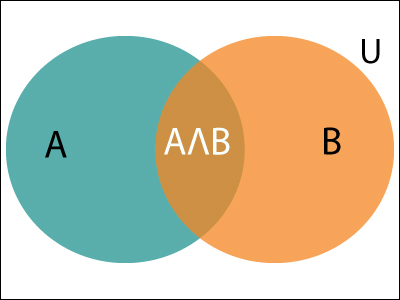
It can be explained by using the below Venn diagram, where B is occurred event, so sample space will be reduced to set B, and now we can only calculate event A when event B is already occurred by dividing the probability of P(A⋀B) by P( B ).

Example:

In a class, there are 70% of the students who like English and 40% of the students who likes English and mathematics, and then what is the percent of students those who like English also like mathematics?

Solution:

Let, A is an event that a student likes Mathematics

B is an event that a student likes English.

Hence, 57% are the students who like English also like Mathematics.

2.10 Probabilities

To make a good decision, an agent cannot simply assume what the world is like and act according to those assumptions. It must consider multiple possible contingencies and their likelihood. Consider the following example.

Example 6.1: Many people consider it sensible to wear a seat belt when traveling in a car because, in an accident, wearing a seat belt reduces the risk of serious injury. However, consider an agent that commits to assumptions and bases its decision on these assumptions. If the agent assumes it will not have an accident, it will not bother with the inconvenience of wearing a seat belt. If it assumes it will have an accident, it will not go out. In neither case would it wear a seat belt! A more intelligent agent may wear a seat belt because the inconvenience of wearing a seat belt is far outweighed by the increased risk of injury or death if it has an accident. It does not stay at home too worried about an accident to go out; the benefits of being mobile, even with the risk of an accident, outweigh the benefits of the extremely cautious approach of never going out. The decisions of whether to go out and whether to wear a seat belt depend on the likelihood of having an accident, how much a seat belt helps in an accident, the inconvenience of wearing a seat belt, and how important it is to go out. The various trade-offs may be different for different agents. Some people do not wear seat belts, and some people do not go out because of the risk of accident.

Reasoning under uncertainty has been studied in the fields of probability theory and decision theory. Probability is the calculus of gambling. When an agent makes decisions and uncertainties are involved about the outcomes of its action, it is gambling on the outcome. However, unlike a gambler at the casino, the agent cannot opt out and decide not to gamble; whatever it does - including doing nothing - involves uncertainty and risk. If it does not take the probabilities into account, it will eventually lose at gambling to an agent that does. This does not mean, however, that making the best decision guarantees a win.

Many of us learn probability as the theory of tossing coins and rolling dice. Although this may be a good way to present probability theory, probability is applicable to a much richer set of applications than coins and dice. In general, we want a calculus for belief that can be used for making decisions.

The view of probability as a measure of belief, as opposed to being a frequency, is known as Bayesian probability or subjective probability. The term subjective does not mean arbitrary, but rather it means "belonging to the subject." For example, suppose there are three agents, Alice, Bob, and Chris, and one die that has been tossed. Suppose Alice observes that the outcome is a "6" and tells Bob that the outcome is even, but Chris knows nothing about the outcome. In this case, Alice has a probability of 1 that the outcome is a "6," Bob has a probability of (1)/(3) that it is a "6" (assuming Bob believes Alice and treats all of the even outcomes with equal probability), and Chris may have probability of (1)/(6) that the outcome is a "6." They all have different probabilities because they all have different knowledge. The probability is about the outcome of this particular toss of the die, not of some generic event of tossing dice. These agents may have the same or different probabilities for the outcome of other coin tosses.

The alternative is the frequentist view, where the probabilities are long-run frequencies of repeatable events. The Bayesian view of probability is appropriate for intelligent agents because a measure of belief in particular situations is what is needed to make decisions. Agents do not encounter generic events but have to make a decision based on uncertainty about the particular circumstances they face.

Probability theory can be defined as the study of how knowledge affects belief. Belief in some proposition, α, can be measured in terms of a number between 0 and 1. The probability α is 0 means that α is believed to be definitely false (no new evidence will shift that belief), and a probability of 1 means that α is believed to be definitely true. Using 0 and 1 is purely a convention.

Adopting the belief view of probabilities does not mean that statistics are ignored. Statistics of what has happened in the past is knowledge that can be conditioned on and used to update belief.

We are assuming that the uncertainty is epistemological - pertaining to an agent's knowledge of the world - rather than ontological - how the world is. We are assuming that an agent's knowledge of the truth of propositions is uncertain, not that there are degrees of truth. For example, if you are told that someone is very tall, you know they have some height; you only have vague knowledge about the actual value of their height.

If an agent's probability of some α is greater than zero and less than one, this does not mean that α is true to some degree but rather that the agent is ignorant of whether α is true or false. The probability reflects the agent's ignorance.

2.11 Bayesian Networks

Bayesian belief network is key computer technology for dealing with probabilistic events and to solve a problem which has uncertainty. We can define a Bayesian network as:

"A Bayesian network is a probabilistic graphical model which represents a set of variables and their conditional dependencies using a directed acyclic graph."

It is also called a Bayes network, belief network, decision network, or Bayesian model.

Bayesian networks are probabilistic, because these networks are built from a probability distribution, and also use probability theory for prediction and anomaly detection.

Real world applications are probabilistic in nature, and to represent the relationship between multiple events, we need a Bayesian network. It can also be used in various tasks including prediction, anomaly detection, diagnostics, automated insight, reasoning, time series prediction, and decision making under uncertainty.

Bayesian Network can be used for building models from data and experts opinions, and it consists of two parts:

• Directed Acyclic Graph
• Table of conditional probabilities.

The generalized form of Bayesian network that represents and solve decision problems under uncertain knowledge is known as an Influence diagram.

A Bayesian network graph is made up of nodes and Arcs (directed links), where:

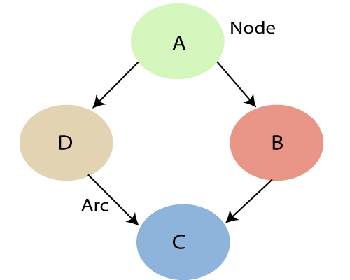
• Each node corresponds to the random variables, and a variable can be continuous or discrete.
• Arc or directed arrows represent the causal relationship or conditional probabilities between random variables. These directed links or arrows connect the pair of nodes in the graph.
  These links represent that one node directly influence the other node, and if there is no directed link that means that nodes are independent with each other
  • In the above diagram, A, B, C, and D are random variables represented by the nodes of the network graph.
  • If we are considering node B, which is connected with node A by a directed arrow, then node A is called the parent of Node B.
  • Node C is independent of node A.

Note: The Bayesian network graph does not contain any cyclic graph. Hence, it is known as a directed acyclic graph or DAG.

The Bayesian network has mainly two components:

• Causal Component
• Actual numbers

Each node in the Bayesian network has condition probability distribution P(Xi |Parent(Xi) ), which determines the effect of the parent on that node.

Bayesian network is based on Joint probability distribution and conditional probability. So let's first understand the joint probability distribution:

Joint probability distribution:

If we have variables x1, x2, x3,....., xn, then the probabilities of a different combination of x1, x2, x3.. Xn, are known as Joint probability distribution.

P[x1, x2, x3,....., xn], it can be written as the following way in terms of the joint probability distribution.

= P[x1| x2, x3,....., xn]P[x2, x3,....., xn]

= P[x1| x2, x3,....., xn]P[x2|x3,....., xn]....P[xn-1|xn]P[xn].

In general for each variable Xi, we can write the equation as:

P(Xi|Xi-1,........., X1) = P(Xi |Parents(Xi ))

Explanation of Bayesian network:

Let's understand the Bayesian network through an example by creating a directed acyclic graph:

Example: Harry installed a new burglar alarm at his home to detect burglary. The alarm reliably responds at detecting a burglary but also responds for minor earthquakes. Harry has two neighbors David and Sophia, who have taken a responsibility to inform Harry at work when they hear the alarm. David always calls Harry when he hears the alarm, but sometimes he got confused with the phone ringing and calls at that time too. On the other hand, Sophia likes to listen to high music, so sometimes she misses to hear the alarm. Here we would like to compute the probability of Burglary Alarm.

Problem:

Calculate the probability that alarm has sounded, but there is neither a burglary, nor an earthquake occurred, and David and Sophia both called the Harry.

Solution:

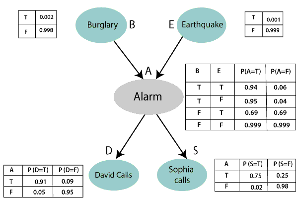
• The Bayesian network for the above problem is given below. The network structure is showing that burglary and earthquake is the parent node of the alarm and directly affecting the probability of alarm's going off, but David and Sophia's calls depend on alarm probability.
• The network is representing that our assumptions do not directly perceive the burglary and also do not notice the minor earthquake, and they also not confer before calling.
• The conditional distributions for each node are given as conditional probabilities table or CPT.
• Each row in the CPT must be sum to 1 because all the entries in the table represent an exhaustive set of cases for the variable.
• In CPT, a boolean variable with k boolean parents contains 2K probabilities. Hence, if there are two parents, then CPT will contain 4 probability values

List of all events occurring in this network:

• Burglary (B)
• Earthquake(E)
• Alarm(A)
• David Calls(D)
• Sophia calls(S)

We can write the events of problem statement in the form of probability: P[D, S, A, B, E], can rewrite the above probability statement using joint probability distribution:

P[D, S, A, B, E]= P[D | S, A, B, E]. P[S, A, B, E]

=P[D | S, A, B, E]. P[S | A, B, E]. P[A, B, E]

= P [D| A]. P [ S| A, B, E]. P[ A, B, E]

= P[D | A]. P[ S | A]. P[A| B, E]. P[B, E]

= P[D | A ]. P[S | A]. P[A| B, E]. P[B |E]. P[E]

Let's take the observed probability for the Burglary and earthquake component:

P(B= True) = 0.002, which is the probability of burglary.

P(B= False)= 0.998, which is the probability of no burglary.

P(E= True)= 0.001, which is the probability of a minor earthquake

P(E= False)= 0.999, Which is the probability that an earthquake not occurred.

We can provide the conditional probabilities as per the below tables:

Conditional probability table for Alarm A:

The Conditional probability of Alarm A depends on Burglar and earthquake:

Conditional probability table for David Calls:

The Conditional probability of David that he will call depends on the probability of Alarm.

Conditional probability table for Sophia Calls:

The Conditional probability of Sophia that she calls is depending on its Parent Node "Alarm."

From the formula of joint distribution, we can write the problem statement in the form of probability distribution:

P(S, D, A, ¬B, ¬E) = P (S|A) *P (D|A)*P (A|¬B ^ ¬E) *P (¬B) *P (¬E).

= 0.75* 0.91* 0.001* 0.998*0.999

= 0.00068045.

Hence, a Bayesian network can answer any query about the domain by using Joint distribution.

The semantics of Bayesian Network:

There are two ways to understand the semantics of the Bayesian network, which is given below:

1. To understand the network as the representation of the Joint probability distribution.

It is helpful to understand how to construct the network.

2. To understand the network as an encoding of a collection of conditional independence statements.

It is helpful in designing inference procedure.

Text Books

1. S. Russell and P. Norvig, “Artificial Intelligence: A Modern Approach,” Prentice Hall

2. E. Rich, K. Knight and S. B. Nair, “Artificial Intelligence,” TMH

References

1. C. Bishop,“Pattern Recognition and Machine Learning," Springer

2. D. W. Patterson, “Introduction to artificial intelligence and expert systems,” Prentice Hall

3. A. C.Staugaard, Jr., “Robotics and AI: An Introduction to Applied Machine Intelligence,” Prentice Hall

4. I. Bratko, “Prolog Programming for Artificial Intelligence,” Addison-Wesley

5. S. O. Haykin, “Neural Networks and Learning Machines,” Prentice Hall

6. D.Jurafsky and J. H. Martin,“Speech and Language Processing,” Prentice Hall