Linear classifiers classify data into labels based on a linear combination of input features. Therefore, these classifiers distinguish data using a line or plane or a hyperplane (a plane with more than 2 dimensions) (a plane in more than 2 dimensions). They can only be used to classify data that is linearly separable. They can be updated to classify non-linearly separable data
Drawbacks of linear classifiers –
● Know what is meant by convexity, and be able to use convexity to prove that a given set of training cases is not linearly separable.
● Understand how we can sometimes still distinguish the groups using a basis function representation.
We will discuss 3 big algorithms in linear binary classification -
- Perceptron:
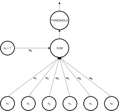
In Perceptron, we take a weighted linear combination of input features and pass it through a thresholding function which outputs 1 or 0. The sign of wTx tells us which side of the plane wTx=0, the point x lies on. Thus by taking threshold as 0, perceptron classifies data depending on which side of the plane the new point lies on.
The task during training is to arrive at the plane (defined by w) that accurately classifies the training data. If the data is linearly separable, perceptron training always converges.
|
Fig 1: perceptron
2. SVM
There may be several hyperplanes that separate linearly separable data. SVM determines the optimum separating hyperplane using principles of geometry.
3. Logistic Regression
Another approach to linear classification is the logistic regression model, which, despite its name, is a classification rather than a regression system.
In Logistic regression, we take a weighted linear combination of input features and pass it through a sigmoid function which outputs a number between 1 and 0. Unlike perceptron, which only tells us which side of the plane the point lies on, logistic regression gives a likelihood of a point lying on a particular side of the plane.
The probability of classification would be very similar to 1 or 0 as the point goes far away from the plane. The chance of classification of points very close to the plane is close to 0.5.
|
Fig 2: logistic regression
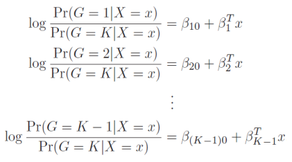
The model is defined in terms of K-1 log-odds ratios, with an arbitrary class chosen as reference class (in this example it is the last class, K) (in this example it is the last class, K). Consequently, the difference between log-probabilities of belonging to a given class and to the reference class is modelled linearly as
where G stands for the real, observed class. From here, the probabilities of an observation belonging to each of the groups can be determined as
that clearly shows that all class probabilities add up to one. |
Logistic regression models are usually calculated by maximum likelihood. Much as linear models for regression can be regularized to increase accuracy, so can logistic regression. In reality, L2 penalty is the default setting. It also supports L1 and Elastic Net penalties (to read more on these, check out the link above), but not all of them are supported by all solvers.
Key takeaway:
● Logistic Regression models the probabilities of an observation belonging to each of the classes through linear functions.
● It is usually considered safer and more stable than discriminant analysis methods, since it is relying on less assumptions.
● It also turned out to be the most accurate for our example spam results.
The approach to be explored is the Linear Discriminant Analysis (LDA).
It assumes that the joint density of all features, conditional on the target's class, is a multivariate Gaussian. This implies that the density P of the features X, given the target y is in class k, are assumed to be given by
|
where d is the number of characteristics, μ is a mean vector, and Σ k the covariance matrix of the Gaussian density for class k.
The decision boundary between two classes, say k and l, is the hyperplane on which the probability of belonging to either class is the same. This means that, on this hyperplane, the difference between the two densities (and hence also the log-odds ratio between them) should be zero.
An significant assumption in LDA is that the Gaussians for different groups share the same covariance matrix: the subscript k from Σ k in the formula above can be dropped. This statement comes in handy for the log-odds ratio calculation: it makes the normalisation factors and certain quadratic sections in the exponent cancel out. This yields a decision boundary between k and l that is linear in X:
|
To measure the density of the features, P(X|y=k), one only has to estimate the Gaussian parameters: the means μ k as the sample means and the covariance matrix Σ as the empirical sample covariance matrix.
|
where P(y=k) is the prior likelihood of belonging to class k and can be determined by the proportion of k-class observations in the sample.
Key takeaway:
● Linear Discriminant Analysis (LDA) assumes that the joint densities of all features given target’s classes are multivariate Gaussians with the same covariance for each class.
● The assumption of common covariance is a strong one, but if accurate, allows for more efficient parameter estimation (lower variance) (lower variance).
● On the other hand, this typical covariance matrix is calculated based on all points, also those far from the decision boundary. This makes LDA vulnerable to outliers.
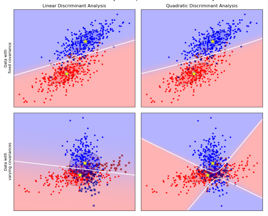
LDA’s assumption that the Gaussians for different classes share the same covariance matrix is convenient, but might be incorrect for particular data. The left column in the picture below shows how LDA performs for data that indeed come from a multivariate Gaussians with a common covariance matrix (upper panel) versus when the data for different classes have different covariances (lower panel) (lower panel).
|
Fig 3: linear and quadratic discriminant analysis
Hence, one might want to relax the common covariance assumption. In this case, there is not one, but k covariance matrices to be estimated. If there are many features, this can lead to a dramatic increase in the number of parameters in the model.
Key takeaway:
● Quadratic Discriminant Analysis (QDA) relaxes the common covariance assumption of LDA by estimating a separate covariance matrix for each class.
● This gives the model more flexibility, but in the case of several features can lead to a drastic increase in the number of parameters in the model.
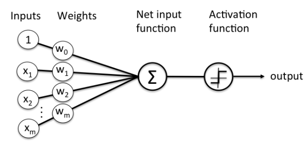
A perceptron is a neural network unit (an artificial neuron) that does certain
computations to detect features or business intelligence in the input data.
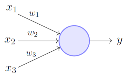
A Perceptron can also be explained as an algorithm for supervised learning of binary classifiers. it enables neurons to learn and processes elements in the training set one at a time.
|
Fig 4: basic perceptron model
There are two types of Perceptrons:
● Single layer Perceptrons can learn only linearly separable patterns.
● Multilayer Perceptrons or feedforward neural networks with two or more layers have greater processing power.
The Perceptron algorithm learns the weights for the input signals in order to draw a
linear decision boundary.
|
Fig 5: schmentic of perceptron
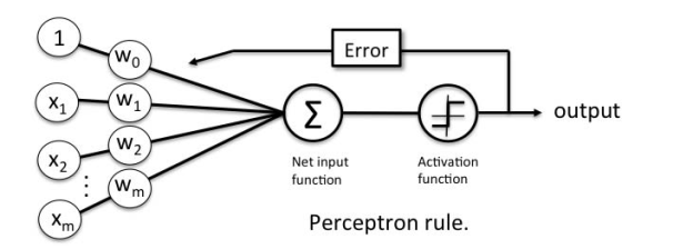
Perceptron Learning Rule
Perceptron Learning Rule states that the algorithm would automatically learn the
optimal weight coefficients. The input features are then multiplied with these weights
to determine if a neuron fires or not.
The Perceptron receives multiple input signals, and if the sum of the input signals
exceeds a certain threshold, it either outputs a signal or does not return an output. In
the context of supervised learning and classification, this can then be used to predict
the class of a sample.
|
Fig 6: perceptron rule
Key takeaway:
● A perceptron is a neural network unit that does certain computations to detect features or business intelligence in the input data.
● A Perceptron can also be explained as an algorithm for supervised learning of binary classifiers.
● Perceptron Learning Rule states that the algorithm would automatically learn the optimal weight coefficients.
● The Perceptron receives multiple input signals, and if the sum of the input signals exceeds a certain threshold, it either outputs a signal or does not return an output.
SVM is another linear classification algorithm (One which separates data with a hyperplane) just like logistic regression and perceptron algorithms.
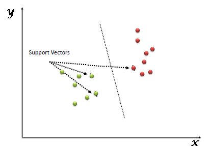
Given any linearly separable data, we can have multiple hyperplanes that can function as a separation boundary as shown. SVM selects the "optimal" hyperplane of all candidate hyperplanes.
|
Fig 7: support vector machine
To understand definition of "optimal" hyperplane, let us first define some concepts we will use
● Margin: It is the distance of the separating hyperplane to its nearest point/points.
● Support Vectors: The point/points closest to the dividing hyperplane.
The optimal hyperplane is defined as the one which maximises the margin. Thus SVM is posed as an optimization problem where we have to maximise margin subject to the constraint that all points lie on the correct side of the separating hyperplane
If all candidate hyperplanes correctly classify the data, why is maximum margin hyperplane the optimal one? One intuitive explanation is - If the incoming samples to be classified contain noise, we do not want them to cross the boundary and be classified incorrectly.
Advantages:
● It works very well with a clear margin of separation
● It is useful in high dimensional spaces.
● It is useful in situations where the number of dimensions is greater than the number of samples.
● It uses a subset of training points in the decision function (called support vectors), so it is also memory efficient.
Disadvantages:
● It doesn’t work well when we have a broad data set because the necessary training time is higher.
● It also doesn’t work very well, when the data set has more noise i.e. target classes are overlapping.
● SVM doesn’t explicitly have probability estimates, these are determined using a costly five-fold cross-validation.
Kernels
Kernels are functions that return without ever calculating given x1 and x2. This means we can convert feature vectors to infinite dimensions and still measure dot products without incurring any additional computational costs!
If you look at the SVM optimization problem's formulation, you'll find that all we ever need is the dot product. The vectors are never needed individually. This makes SVM simple to solve, even though the features are translated into infinite dimensions.
Assume we need a transformation.
In this case, the kernel function is simply (x1 + x2)2. As a consequence, rather than multiplying all terms, we can simply calculate x1 + x2 as a number and square it. To calculate the dot product, there was no need to calculate the higher dimensional phi (x) explicitly. Consider what would happen if the projection was done in 100 dimensions rather than three. Finding a kernel function like this would make computations a lot easier.
Let's take a look at a polynomial kernel of degree 2 as an example.
Instead of calculating the full expanded version of the dot product, we simply need to square 1 + x1x2. |
Key takeaway:
● SVM is another linear classification algorithm (One which separates data with a hyperplane) just like logistic regression and perceptron algorithms.
● SVM selects the "optimal" hyperplane of all candidate hyperplanes.
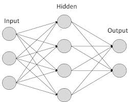
Neural networks are mathematical models that use learning algorithms inspired by
the brain to store information. Since neural networks are used in machines, they are
collectively called an ‘artificial neural network.’
|
Fig 8: Artificial neural network
Nowadays, the term machine learning is often used in this field and is the scientific
discipline that is concerned with the design and development of algorithms that allow computers to learn, based on data, such as from sensor data or databases.
A major focus of machine-learning research is to automatically learn to recognize complex patterns and make intelligent decisions based on data. Hence, machine learning is closely related to fields such as statistics, data mining, pattern recognition, and artificial intelligence.
Neural networks are a popular framework to perform machine learning, but there are
many other machine-learning methods, such as logistic regression, and support
vector machines.
Types of Artificial Neural Networks
● FeedForward
● Feedback.
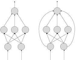
FeedForward ANN - In this ANN:
● information flow is unidirectional
● A unit sends information to other unit from which it does not receive any
information.
● No feedback loops.
● Used in pattern generation/recognition/classification.
● Have fixed inputs and outputs.
|
Fig 9: feed forward ANN
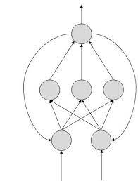
FeedBack ANN
● feedback loops are allowed.
● used in content addressable memories.
|
Fig 10: feedback ANN
Back Propagation
The Backpropagation Algorithm is based on generalizing the Widrow-Hoff learning
rule. It uses supervised learning, which means that the algorithm is provided with
examples of the inputs and outputs that the network should compute, and then the
error is calculated.
The backpropagation algorithm starts with random weights, and the goal is to adjust
them to reduce this error until the ANN learns the training data.
Standard backpropagation is a gradient descent algorithm in which the network
weights are moved along the negative of the gradient of the performance function.
The combination of weights that minimizes the error function is considered a solution
to the learning problem.
The backpropagation algorithm requires a differentiable activation function, and the
most commonly used are tan-sigmoid, log-sigmoid, and, occasionally, linear. Feed-
forward networks often have one or more hidden layers of sigmoid neurons followed
by an output layer of linear neurons. This structure allows the network to learn
nonlinear and linear relationships between input and output vectors. The linear
the output layer lets the network get values outside the range − 1 to + 1.
For the learning process, the data must be divided in two sets:
training data set, which is used to calculate the error gradients and to update
the weights; Validation data set, which allows selecting the optimum number of iterations to avoid overlearning.
As the number of iterations increases, the training error reduces whereas the
validation data set error begins to drop, then reaches a minimum and finally
increases. Continuing the learning process after the validation error arrives at a
minimum leads to overlearning. Once the learning process is finished, another data
set (test set) is used to validate and confirm the prediction accuracy.
Properly trained backpropagation networks tend to give reasonable answers when
presented with new inputs.Usually, in ANN approaches, data normalization is
necessary before starting the training process to ensure that the influence of the
input variable in the course of model building is not biased by the magnitude of its
native values, or its range of variation. The normalization technique, usually consists
of a linear transformation of the input/output variables to the range (0, 1).
Feedforward Dynamics
When a Back Propagation network is cycled, the activations of the input units are
propagated forward to the output layer through the connecting weights. As in
perceptron, the net input to a unit is determined by the weighted sum of its inputs:
netj = Σi wjiai where a i is the input activation from unit i and w ji is the weight connecting unit i to unit j. However, instead of calculating a binary output, the net input is added to the unit’s bias and the resulting value is passed through a sigmoid function:
The bias term plays the same role as the threshold in the perceptron. But unlike binary output of the perceptron, the output of a sigmoid is a continuous real-value between 0 and 1. The sigmoid function is sometimes called a “squashing” function because it maps its inputs onto a fixed range. |
Key takeaway:
● Neural networks are mathematical models that use learning algorithms inspired by the brain to store information.
● A major focus of machine-learning research is to automatically learn to recognize complex patterns and make intelligent decisions based on data.
● Neural networks are a popular framework to perform machine learning, but there are many other machine-learning methods, such as logistic regression, and support vector machines.
● The Backpropagation Algorithm is based on generalizing the Widrow-Hoff learning rule.
● The backpropagation algorithm starts with random weights, and the goal is to adjust them to reduce this error until the ANN learns the training data.
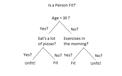
Decision Tree is a Supervised learning technique that can be used for both
classification and Regression problems, but mostly it is preferred for solving
Classification problems. It is a tree-structured classifier, where internal nodes
represent the features of a dataset, branches represent the decision rules and each
leaf node represents the outcome.
|
Fig 11: decision tree example
In a Decision tree can be divided into:
● Decision Node
● Leaf Node
Decision nodes are marked by multiple branches that represent different decision
conditions whereas output of those decisions is represented by leaf node and do not
contain further branches.
The decision tests are performed on the basis of features of the given dataset.
It is a graphical representation for getting all the possible solutions to a problem/decision based on given conditions.
Decision Tree algorithm:
● Comes under the family of supervised learning algorithms.
● Unlike other supervised learning algorithms, decision tree algorithms can be used for solving regression and classification problems.
● Are used to create a training model that can be used to predict the class or value of the target variable by learning simple decision rules inferred from prior data (training data).
● Can be used for predicting a class label for a record we start from the root of the tree.
● Values of the root attribute are compared with the record’s attribute. On the basis of comparison, a branch corresponding to that value is considered and jumps to the next node.
Issues in Decision tree learning
● It is less appropriate for estimation tasks where the goal is to predict the value of a continuous attribute.
● This learning is prone to errors in classification problems with many classes and relatively small number of training examples.
● This learning can be computationally expensive to train. The process of growing a decision tree is computationally expensive. At each node, each candidate splitting field must be sorted before its best split can be found. In some algorithms, combinations of fields are used and a search must be made for optimal combining weights. Pruning algorithms can also be expensive since many candidate sub-trees must be formed and compared.
- Avoiding overfitting
A decision tree’s growth is specified in terms of the number of layers, or depth, it’s allowed to have. The data available to train the decision tree is split into training and testing data and then trees of various sizes are created with the help of the training data and tested on the test data. Cross-validation can also be used as part of this approach. Pruning the tree, on the other hand, involves testing the original tree against pruned versions of it. Leaf nodes are removed from the tree as long as the pruned tree performs better on the test data than the larger tree.
Two approaches to avoid overfitting in decision trees:
● Allow the tree to grow until it overfits and then prune it.
● Prevent the tree from growing too deep by stopping it before it perfectly classifies the training data.
2. Incorporating continuous valued attributes
3. Alternative measures for selecting attributes
● Prone to overfitting.
● Require some kind of measurement as to how well they are doing.
● Need to be careful with parameter tuning.
● Can create biased learned trees if some classes dominate.
Key takeaway:
● Decision Tree is a Supervised learning technique that can be used for both
classification and Regression problems, but mostly it is preferred for solving
Classification problems.
● It is a tree-structured classifier, where internal nodes represent the features of a dataset, branches represent the decision rules and each leaf node represents the outcome.
The Bayes Optimal Classifier is a probabilistic model that predicts the most possible outcome for a new scenario.
The Bayes Theorem, which provides a principled way of estimating a conditional probability, is used to explain it. It's also related to Maximum a Posteriori (MAP), a probabilistic method for determining the most likely hypothesis for a training dataset.
In practice, computing the Bayes Optimal Classifier is computationally costly, if not difficult, and instead, simplifications like the Gibbs algorithm and Naive Bayes can be used to estimate the result.
The Bayes optimal classifier is a probabilistic model that makes the most probable prediction for a new example, given the training dataset.
This model is often referred to as the Bayes optimal learner, the Bayes classifier, Bayes optimal decision boundary, or the Bayes optimal discriminant function.
Bayes Classifier: A probabilistic model that predicts the most possible outcome for new data.
Any model that uses this equation to classify examples is a Bayes optimal classifier, and no other methodology can outperform it on average.
A Bayes optimal classifier, or Bayes optimal learner, is a method that classifies new instances according to [the equation]. On average, no other classification system that uses the same hypothesis space and prior information as this method will outperform it.
It means that any other algorithm that works with the same data, hypotheses, and prior probabilities cannot outperform this method on average. As a consequence, the term "optimal classifier" was coined.
Despite the fact that the classifier allows the best predictions, it isn't flawless due to the ambiguity in the training data and the problem domain and hypothesis space's incomplete coverage. As a consequence, the model will make mistakes. Bayes errors are the name given to these types of errors.
The Bayes error rate is the lowest possible test error rate provided by the Bayes classifier. [...] The irreducible error rate is analogous to the Bayes error rate.
The Bayes error is the smallest possible error that can be made since the Bayes classifier is optimal.
The Bayes Error is the smallest possible error when making predictions.
Key takeaway:
● The Bayes Optimal Classifier is a probabilistic model that predicts the most possible outcome for a new scenario.
● The Bayes optimal classifier is a probabilistic model that makes the most probable prediction for a new example, given the training dataset.
The Naïve Bayes algorithm is comprised of two words Naïve and Bayes, Which can
be described as:
● Naïve: It is called Naïve because it assumes that the occurrence of a certain feature is independent of the occurrence of other features. Such as if the fruit is identified based on color, shape, and taste, then red, spherical, and sweet fruit is recognized as an apple. Hence each feature individually contributes to identifying that it is an apple without depending on each other.
● Bayes: It is called Bayes because it depends on the principle of Bayes’ Theorem.
Naïve Bayes Classifier Algorithm
Naïve Bayes algorithm is a supervised learning algorithm, which is based on the
Bayes theorem and used for solving classification problems. It is mainly used in text
classification that includes a high-dimensional training dataset.
Naïve Bayes Classifier is one of the simple and most effective Classification algorithms which help in building fast machine learning models that can make quick predictions.
It is a probabilistic classifier, which means it predicts based on the probability of an
Object.
Some popular examples of the Naïve Bayes Algorithm are spam filtration,
Sentimental analysis, and classifying articles.
Bayes’ Theorem:
● Bayes’ theorem is also known as Bayes’ Rule or Bayes’ law, which is used to determine the probability of a hypothesis with prior knowledge. It depends on the conditional probability.
● The formula for Bayes’ theorem is given as:
|
Where,
● P(A|B) is Posterior probability: Probability of hypothesis A on the observed event B.
● P(B|A) is Likelihood probability: Probability of the evidence given that the probability of a hypothesis is true.
● P(A) is Prior Probability: Probability of hypothesis before observing the evidence.
● P(B) is a Marginal Probability: Probability of Evidence.
Working of Naïve Bayes’ Classifier can be understood with the help of the below example:
Suppose we have a dataset of weather conditions and corresponding target variable
“Play”. So using this dataset we need to decide whether we should play or not on a
particular day according to the weather conditions. So to solve this problem, we need to follow the below steps:
Convert the given dataset into frequency tables.
Generate a Likelihood table by finding the probabilities of given features.
Now, use Bayes theorem to calculate the posterior probability.
Problem: If the weather is sunny, then the Player should play or not?
Solution: To solve this, first consider the below dataset:
Outlook Play
0 Rainy Yes
1 Sunny Yes
2 Overcast Yes
3 Overcast Yes
4 Sunny No
5 Rainy Yes
6 Sunny Yes
7 Overcast Yes
8 Rainy No
9 Sunny No
10 Sunny Yes
11 Rainy No
12 Overcast Yes
13 Overcast Yes
Frequency table for the Weather Conditions:
Weather Yes No
Overcast 5 0
Rainy 2 2
Sunny 3 2
Total 10 5
Likelihood table weather condition:
Weather No Yes
Overcast 0 5 5/14 = 0.35
Rainy 2 2 4/14 = 0.29
Sunny 2 3 5/14 = 0.35
All 4/14=0.29 10/14=0.71
Applying Bayes’ theorem:
P(Yes|Sunny)= P(Sunny|Yes)*P(Yes)/P(Sunny)
P(Sunny|Yes)= 3/10= 0.3
P(Sunny)= 0.35
P(Yes)=0.71
So P(Yes|Sunny) = 0.3*0.71/0.35= 0.60
P(No|Sunny)= P(Sunny|No)*P(No)/P(Sunny)
P(Sunny|NO)= 2/4=0.5
P(No)= 0.29
P(Sunny)= 0.35
So P(No|Sunny)= 0.5*0.29/0.35 = 0.41
So as we can see from the above calculation that P(Yes|Sunny)>P(No|Sunny)
Hence on a Sunny day, the Player can play the game.
Advantages of Naïve Bayes Classifier:
● Naïve Bayes is one of the fast and easy ML algorithms to predict a class of datasets.
● It can be used for Binary as well as Multi-class Classifications.
● It performs well in Multi-class predictions as compared to the other Algorithms.
● It is the most popular choice for text classification problems.
Disadvantages of Naïve Bayes Classifier:
● Naive Bayes assumes that all features are independent or unrelated, so it cannot learn the relationship between features.
Applications of Naïve Bayes Classifier:
● It is used for Credit Scoring.
● It is used in medical data classification.
● It can be used in real-time predictions because Naïve Bayes Classifier is an eager
● learner.
● It is used in Text classification such as Spam filtering and Sentiment analysis.
Types of Naïve Bayes Model:
There are three types of Naive Bayes Model, which are given below:
Gaussian: The Gaussian model assumes that features follow a normal distribution.
This means if predictors take continuous values instead of discrete, then the model
assumes that these values are sampled from the Gaussian distribution.
Multinomial: The Multinomial Naïve Bayes classifier is used when the data is
multinomial distributed. It is primarily used for document classification problems, it
means a particular document belongs to which categories such as Sports, Politics,
education, etc.
The classifier uses the frequency of words for the predictors.
Bernoulli: The Bernoulli classifier works similarly to the Multinomial classifier, but the predictor variables are the independent Booleans variables. Such as if a particular word is present or not in a document. This model is also famous for document classification tasks.
Key takeaway:
● Naïve Bayes algorithm is a supervised learning algorithm, which is based on the Bayes theorem and used for solving classification problems.
● Naïve Bayes Classifier is one of the simple and most effective Classification algorithms which help in building fast machine learning models that can make quick predictions.
● Bayes’ theorem is also known as Bayes’ Rule or Bayes’ law, which is used to determine the probability of a hypothesis with prior knowledge.
References:
- Introduction to Machine Learning Edition 2, by Ethem Alpaydin.
2. Understanding Machine Learning. Shai Shalev-Shwartz and Shai Ben-David. Cambridge University Press. 2017. [SS-2017]
3. The Elements of Statistical Learning. Trevor Hastie, Robert Tibshirani and Jerome Friedman. Second Edition. 2009. [TH-2009]
