Unit-4
Hypothesis testing
Hypothesis testing is a mathematical method for making statistical decisions based on evidence from experiments. Hypothesis testing is simply making an inference about a population parameter.
Hypothesis testing is the process of using statistical tests on a sample to draw inferences or conclusions about the overall population or data. T-test, which I will address in this tutorial, is used to draw the same inferences for various machine learning models.
We must make certain assumptions in order to draw some inferences, which leads to two concepts that are used in hypothesis testing.
● Null hypothesis: The null hypothesis refers to the belief that no anomaly trend occurs or to believing in the assumption made.
● Alternate hypothesis: Contrary to the null hypothesis, it indicates that observation is the result of a real effect.
P Values
It can also be used in machine learning algorithms as proof or a degree of significance for the null hypothesis. It is the value of the predictors in relation to the target.
In comparison, if the p-value in a machine learning model against an independent variable is less than 0.05, the variable is taken into account, implying that there is heterogeneous behavior with the target that is useful and can be learned by machine learning algorithms.
The following are the steps involved in hypothesis testing:
● Assume a null hypothesis; in most machine learning algorithms, no anomaly exists between the target and the independent variable.
● Obtain a sample
● Calculate the test results.
● Decide whether the null hypothesis should be accepted or rejected.
Error
Because of the scarcity of data resources, hypothesis testing is done on a sample of data rather than the entire population. Hypothesis testing can result in errors due to inferences drawn from sample data, which can be divided into two categories:
● Type I Error: We reject the null hypothesis when it is true in this error.
● Type II Error: We accept the null hypothesis when it is false in this error.
Ensemble methods are a type of machine learning technique that combines multiple base models to construct a single best-fit predictive model.
Ensemble methods are meta-algorithms that incorporate many machine learning techniques into a single predictive model to minimize uncertainty (bagging), bias (boosting), or increase prediction accuracy (stacking).
The methods used in ensembles can be divided into two categories:
- The base learners are created sequentially in sequential ensemble methods (e.g. AdaBoost).
The primary motive for sequential approaches is to take advantage of the base learners' interdependence. By giving previously mislabeled examples more weight, the overall performance can be improved.
2. The base learners are generated in parallel using parallel ensemble methods (e.g. Random Forest).
The primary reason for parallel approaches is to take advantage of the independence between the base learners because averaging will significantly reduce error.
The majority of ensemble methods employ a single base learning algorithm to generate homogeneous base learners, or learners of the same kind, resulting in homogeneous ensembles.
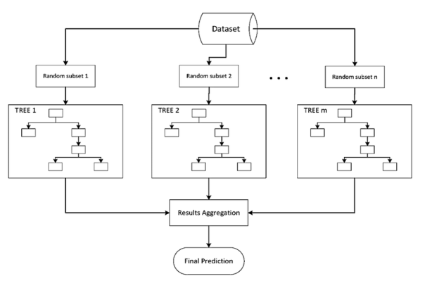
Bootstrap aggregation is referred to as "bagging." Averaging several estimates together is one way to reduce the uncertainty of an estimate. For example, we can compute the ensemble by training M different trees on different subsets of the data.
|
To collect data subsets for training the base learners, bagging employs bootstrap sampling. Bagging uses voting for classification and averaging for regression to combine the outputs of base learners.
Bootstrap Aggregating, or Bagging. The term Bagging comes from the fact that it incorporates Bootstrapping and Aggregation into a single ensemble model. Multiple bootstrapped subsamples are taken from a sample of data. On each of the bootstrapped subsamples, a Decision Tree is formed. An algorithm is used to aggregate over the Decision Trees to form the most efficient predictor after each subsample Decision Tree has been created.
|
Fig 1: example of bagging sample
Adaboost
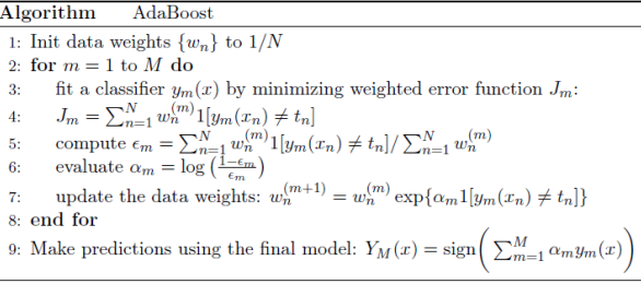
Adaptive Boosting, or AdaBoost, is a method of combining many weak learners to create a strong learner. A weak learner is a learning algorithm that outperforms random guessing on a consistent basis. AdaBoost brings together a group of these learners to form a hypothesis with arbitrarily high accuracy. AdaBoost is an adaptive algorithm, which means it learns from its mistakes.
The AdaBoost algorithm, which stands for adaptive boosting, is the most widely used form of boosting algorithm.
|
Gradient Tree Boosting is a generalization of boosting for loss functions that are differentiable in any way. It can be used to solve problems involving regression and classification. Gradient Boosting is a method of constructing a model in a sequential manner.
|
Given the current model Fm-1(x), the decision tree hm(x) is chosen at each stage to minimize a loss function L:
|
The type of loss function used in regression and classification algorithms differs.
Key takeaway:
● Bootstrap aggregation is referred to as "bagging." Averaging several estimates together is one way to reduce the uncertainty of an estimate.
● The AdaBoost algorithm, which stands for adaptive boosting, is the most widely used form of boosting algorithm.
● Gradient Tree Boosting is a generalization of boosting for loss functions that are differentiable in any way.
Clustering is the process of grouping data. Based on some similarity measure, the resulting groups should be such that data within the same group should be identical and data within different groups should be dissimilar. A good clustering algorithm can create groups that maximize data similarity among similar groups while minimizing data similarity among different groups.
Application of clustering
Classes are conceptually important groups of objects with identical characteristics. Data that is defined in terms of classes offers a better image than raw data.
A image, for example, may be defined as "a picture of houses, vehicles, and people" or by specifying the pixel value. The first approach is more useful for finding out what the picture is about.
Clustering is also seen as a prelude to more sophisticated data processing techniques.
As an example,
● A music streaming service could divide users into groups based on their musical preferences. Instead of estimating music recommendations for each individual person, these classes can be measured. It's also simpler for a new consumer to find out who their closest neighbors are.
● Time is proportional to n2 in linear regression, where n is the number of samples. As a result, nearby data points may be grouped together as a single representative point in large datasets. On this smaller dataset, regression can be used.
● There may be millions of colors in a single picture. To make the color palette smaller, identical RGB values could be grouped together.
Types of groups of clusters
Cluster classes are classified into four categories:
● Partitional - A series of non-overlapping clusters. There is only one cluster per each data point.
● Hierarchical - Clusters have sub-clusters in a hierarchical system.
● Overlapping - A data point may belong to multiple clusters, which means the clusters overlap.
● Fuzzy - Each data point is assigned a weight and belongs to one of the clusters. If there are five clusters, each data point belongs to all five clusters and is assigned five weights. The sum of these weights is 1.
Types of clusters
Depending on the issue at hand, clusters may be of various forms. Clusters can be anything from
● Well separated clusters
Each data point in a well-separated cluster is closer to all points within the cluster than to any point outside of it. When clusters are well apart, this is more likely to occur.
● Prototype based clusters
Each cluster in prototype-based clusters is represented by a single data point. Clusters are allocated to data points. Each point in a cluster is closer to that cluster's representative than any other cluster's representative.
● Graph based clusters
A cluster is a group of linked data points that do not have a connection to any point outside the cluster if data is described as a graph with nodes as data points and edges as connections. Depending on the issue, the word "related" can mean various things.
● Density based clusters
A density-based cluster is a dense set of data points surrounded by a low-density area.
Key takeaway:
● Clustering is the process of grouping data. Based on some similarity measure, the resulting groups should be such that data within the same group should be identical and data within different groups should be dissimilar.
● A good clustering algorithm can create groups that maximize data similarity among similar groups while minimizing data similarity among different groups.
For numeric results, K-Means clustering is one of the most commonly used prototype-based clustering algorithms. The centroid or mean of all the data points in a cluster is the prototype of a cluster in k-means. As a consequence, the algorithm works best with continuous numeric data. When dealing with data that includes categorical variables or a mixture of quantitative and categorical variables.
Pseudo Algorithm
- Choose an appropriate value of K (number of clusters we want)
- Generate K random points as initial cluster centroids
- Until convergence (Algorithm converges when centroids remain the same between iterations):
● Assign each point to a cluster whose centroid is nearest to it ("Nearness" is measured as the Euclidean distance between two points)
● Calculate new values of centroids of each cluster as the mean of all points assigned to that cluster
K-Means as an optimization problem
Any learning algorithm has the aim of minimizing a cost function. We'll see how, by using centroid as a cluster prototype, we can minimize a cost function called "sum of squared error".
|
The sum of squared error is the square of all points' distances from their respective cluster prototypes.
We get by taking the partial derivative of the cost function with respect to and cluster prototype and equating it to 0.
|
Cluster centroids are thus the prototypes that minimize the cost function.
Key takeaway:
● K-Means clustering is one of the most commonly used prototype-based clustering algorithms.
● The algorithm works best with continuous numeric data.
● When dealing with data that includes categorical variables or a mixture of quantitative and categorical variables.
● K-Means is a more effective algorithm. Defining distances between each diamond takes longer than computing a mean.
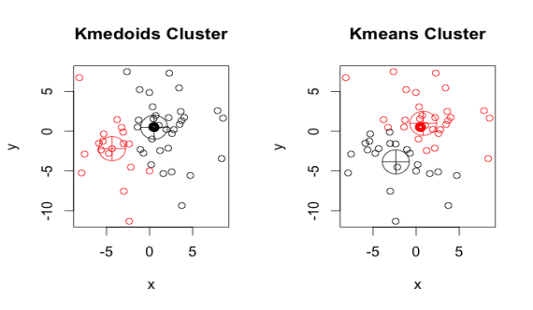
Similar to the k-means algorithm, the k-medoid or PAM(Partitioning Around Medoids) algorithm is a clustering algorithm. A medoid is an object in a cluster whose average dissimilarity to all other objects in the cluster is minimal, i.e., it is the cluster's most centrally located point.
|
Fig 2: K medoids and k means
Kaufman and Rousseeuw introduced the K-Medoids (also known as Partitioning Around Medoid) algorithm in 1987. A medoid is a point in a cluster whose dissimilarities with all other points in the cluster are the smallest.
E = |Pi - Ci| is used to measure the dissimilarity of the medoid(Ci) and object(Pi).
In the K-Medoids algorithm, the cost is given as
|
Algorithm
- Initialize: select k random points out of the n data points as the medoids.
- Associate each data point to the closest medoid by using any common distance metric methods.
- While the cost decreases:
For each medoid m, for each data o point which is not a medoid:
● Swap m and o, associate each data point to the closest medoid, recompute the cost.
● If the total cost is more than that in the previous step, undo the swap.
Similarities between K means and K medoids
● Clustering algorithms and unsupervised machine learning algorithms are also used.
● Both the k-means and k-medoids algorithms are based on partitioning (dividing a dataset into groups) and seek to reduce the distance between points labeled in a cluster and the cluster's center.
Advantages
● It's easy to comprehend and put into effect.
● The K-Medoid Algorithm is a fast algorithm that converges in a predetermined number of steps.
● Other partitioning algorithms are more sensitive to outliers than PAM.
Disadvantages
● The key downside of K-Medoid algorithms is that they are unsuccessful at clustering non-spherical (arbitrary-shaped) groups of objects. This is because it clusters by minimizing the distances between non-medoid objects and the medoid (the cluster center) – in other words, it clusters by compactness rather than connectivity.
● Since the first k medoids are chosen at random, it can yield different results for different runs on the same dataset.
Key takeaway:
● it is less susceptible to outliers, K-Medoids is more stable.
● A medoid is an object in a cluster whose average dissimilarity to all other objects in the cluster is minimal, i.e., it is the cluster's most centrally located point.
DBSCAN (Density Dependent Spatial Clustering of Applications with Noise) is a dense clustering algorithm that is both simple and efficient. Clustering algorithms based on density classify high-density areas separated by low-density areas.
Fundamentally, all clustering approaches use the same approach: we quantify similarities first, then use them to group or batch the data points.
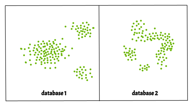
Clusters are dense regions in the data space that are separated by low-density regions. The DBSCAN algorithm is built around the principles of "clusters" and "noise." The main principle is that the neighborhood of a given radius must contain at least a certain number of points for each point of a cluster.
|
Fig 3: different database
Pseudo Algorithm
Given the dataset
- Label all points as core or non core
- Until all core points are visited:
● Add one of non visited core point P to a new cluster
● Until all points in cluster are visited:
○ For each non visited core point P within the cluster
■ Add all core points within boundary of P to the cluster
■ Mark P as visited
3. Until all non-core points are visited:
● If a non core point P has a core point within its boundary, add it to the cluster corresponding to that core point. Else ignore.
DBSCAN algorithm requires two parameters –
- eps : It determines a data point's neighborhood, i.e. if the distance between two points is less than or equal to 'eps,' they are called neighbors. If the eps value is set too low, a considerable portion of the data would be listed as outliers. If it's set to a large value, the clusters will converge and the majority of the data points will be in the same cluster. The k-distance graph is one method for calculating the eps value.
2. MinPits : Within an eps radius, the minimum number of neighbors (data points) is necessary. The larger the dataset, the higher the MinPts value that must be selected. MinPts >= D+1 is a general rule for calculating the minimum MinPts from the number of dimensions D in the dataset. MinPts must have a minimum value of at least 3.
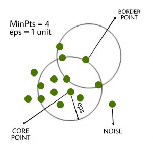
There are three types of data points in this algorithm.
● Core points : If a point has more than MinPts points within eps, it is called a core point.
● Border points : A border point is a point within eps that has less than MinPts but is similar to a core point.
● Noise or Outlier : A point that is not a central point or a boundary point is called a noise or outlier.
|
Fig 4: show three types of data
Advantages of DBSCAN
● Unlike K-means, DBSCAN does not require prior knowledge of the number of clusters.
● DBSCAN can construct clusters of any form, while k-means can only manage globular clusters.
● Only two parameters (R and N) are necessary for DBSCAN, and there are efficient methods for estimating good values for those parameters.
● DBSCAN is noise-resistant.
Key takeaway:
● DBSCAN (Density Dependent Spatial Clustering of Applications with Noise) is a dense clustering algorithm that is both simple and efficient.
● Clustering algorithms based on density classify high-density areas separated by low-density areas.
● The DBSCAN algorithm is built around the principles of "clusters" and "noise."
Spectral Clustering is a rapidly evolving clustering algorithm that has outperformed many conventional clustering algorithms in many situations. It converts the clustering problem into a graph partitioning problem by treating each data point as a graph node.
There are three basic steps in a typical implementation: -
- Building the Similarity Graph : The Similarity Graph is built in the form of an adjacency matrix, which is represented by A, in this step. The following methods can be used to construct the adjacency matrix:-
● Epsilon-neighborhood Graph: The epsilon parameter is set in advance. Then each point is related to all the other points in its epsilon-radius. When the measurements of all the distances between two points are identical, the weights of the edges, i.e. the distance between the two points, are usually not stored because they provide no additional details. As a consequence, the graph constructed in this case is undirected and unweighted.
● K-Nearest Neighbors: A fixed parameter, k, is set up ahead of time. Then, only if v is one of u's k-nearest neighbors, an edge is directed from u to v for two vertices u and v. It's worth noting that this results in the creation of a weighted and directed graph because it's not always the case that each u has v as one of its k-nearest neighbors, and vice versa. Each of the following methods is used to render this graph undirected: -
○ If either v is among u's k-nearest neighbours OR u is among v's k-nearest neighbours, direct an edge from u to v and from v to u.
○ If v is among u's k-nearest neighbors AND u is among v's k-nearest neighbors, direct an edge from u to v and from v to u.
● Fully-Connected Graph: Each point in this graph is connected to every other point by an undirected edge that is weighted by the distance between the two points. Since this method is used to model local neighborhood relationships, the distance is normally determined using the Gaussian similarity metric.
2. Projecting the data onto a lower Dimensional Space: This move is taken to account for the possibility that members of the same cluster may be separated by a significant distance in the dimensional space. As a consequence, the dimensional space is reduced, and some points are closer in the reduced dimensional space, allowing a conventional clustering algorithm to cluster them together. The Graph Laplacian Matrix is used to achieve this. The degree of a node must first be specified before it can be computed. The ith node's degree is given by
|
The edge between the nodes I and j as defined in the adjacency matrix is w ij.
3. Clustering the data : The majority of this method requires clustering the reduced data using any conventional clustering strategy, most commonly K-Means Clustering. Second, a row of the normalized Graph Laplacian Matrix is assigned to each node. The data is then clustered using any regular form. The node identifier is held when transforming the clustering result.
Key takeaway:
● Spectral Clustering is a rapidly evolving clustering algorithm that has outperformed many conventional clustering algorithms in many situations.
● It converts the clustering problem into a graph partitioning problem by treating each data point as a graph node.
References:
- Machine Learning. Tom Mitchell. First Edition, McGraw- Hill, 1997
- P. Langley, Elements of Machine Learning, Morgan Kaufmann, 1995

