UNIT 6

GENERAL MOTION

6.1 General Planar motion

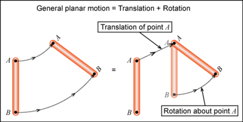
General plane motion of a rigid body refers to a combination of translation and rotation motion.

General planar motion refers to the simultaneous rotational and translational motion of a planar body in a 2-D plane.

General planar motion can be fully specified by knowing both the angular rotation of a line fixed in the body and the motion of any point on the body.

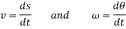
These motions can be related by using a rectilinear position coordinate s to locate the point along its path and an angular position coordinate to specify the orientation of the line. Then these two coordinates are related using the geometry of the problem. The following relation is found.

Differentiating the above equation, gives the relation between velocity and angular velocity .

Where,

Then again differentiating, it yields to the relation between acceleration and angular acceleration

Where,

Application: General Plane Motion

With the case of planar fixed axis rotation dealt with, we turn now to the more complex situation of general plane motion. Recall, once again, that the motion of an arbitrary rigid body can be reduced to the superposition of a translation and a fixed axis rotation. Handling the translation of a rigid body is trivial, all points of the body move with the same velocity and acceleration, and we now know how to deal with fixed axis rotations. Therefore, all that remains is to understand how the two are superposed. As we will find out, this is quite simple.

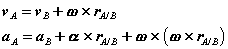
We proceed by returning to the equations we had derived for the arbitrary motion of a rigid body. Recall that these related the velocity  and acceleration  of a point A in the body to the translational motion of an arbitrary reference point B ( and ), and the absolute rotational motion of the body ( and ) as,

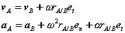
As in the case of fixed axis rotation we simplify these expressions by introducing a set of n-t coordinates. Unlike those used previously, however, the coordinates introduced here refer to the motion of A relative to the reference at B. Therefore,  is directed towards point B, the center of the relative motion, and  is directed along , tangent to the path of A relative to B.

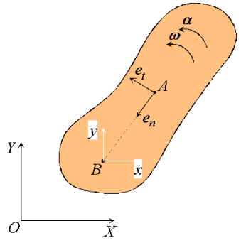
Figure: n-t coordinates for general plane motion.

Substituting, we obtain a simplified expression for the velocity of point A,

Which can be recognized as a superposition of translational and rotational components, each of which we understand very well.

Figure : Decomposition of the absolute velocity of point A.

Proceeding in an analogous way for the acceleration,

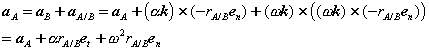
Or,

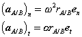
With normal and tangential accelerations of the form,

Therefore, like the velocity, the acceleration of A is a superposition of translational and rotational components. While the normal component is directed along , towards the axis of the rotational motion of A relative to B, the tangential component is directed along , tangent to the path of A relative to B.

Figure : Decomposition of the absolute acceleration of point A.

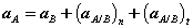
For the general plane motion of a rigid body:

Alternately,

Where  is the position vector of A relative to the reference at B, ,  are the velocity and acceleration of the reference and ,  are the angular velocity and acceleration of the body.

6.2 Free or steady precession

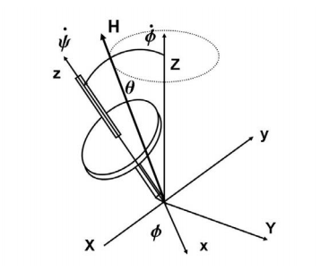
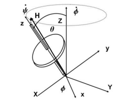
Steady Precession: Gyroscopic Motion We now consider the steady precession of a top about the Z axis. In terms of the variables we have defined, the top rotates with spin velocity ψ˙ about its principal axis, and precesses with angular velocity φ˙ while maintaining a constant angle θ with the vertical axis Z. We then have

φ˙ = constant = φ˙ 0 φ¨ = 0

θ = constant = θ0 θ ˙ = ¨θ = 0

ψ˙ = 0 ψ¨ = 0

For a steady precession of a top, Euler’s equations reduce to

Φ sinθ (I(φ cos θ ˙ + ψ˙) − I0φcosθ) = Mx = MgsinθzG

Note that sinθ cancels, resulting in

Iφψ˙ − (I0 − I) φ˙2cosθ = MgzG

In the usual case for tops or gyroscopes, we have ψ >> φ˙ so that φ˙2 may be ignored. Therefore, for steady precession, the relationship between the precession angular velocity and the spin angular velocity is

φ˙ = MgzG/(Iψ˙)

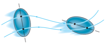
Where I = Izz, the moment of inertia of the gyroscope about its spin axis. This result is also true if θ = 0. For this motion, the angular momentum vector is not aligned with the Z axis as for free-body motion, but is in the plane of z, Z, and rotates around the Z axis according to the applied external moment which is constant and in the x direction. In the limit as ψ˙ >> φ the angular momentum vector is essentially along the axis of ˙ rotation, z, with a slight component due to φ˙ which can be calculated after ψ˙ has been determined. Some attempt to sketch this is shown in the figure, but even this small correction is an approximation for ψ˙ >> φ.˙ F ˙ or ψ >> φ˙,

This same result can be obtained by less complex approach, but it is important to realize that this is an approximation. For the spin velocity much greater than the precessional velocity, we may take the angular momentum vector as directed along the spin or z axis,

H = Iω k. Then the applied moment will process the vector with rotation rate

Ω × H. Since Ω = ΩK = φK, (where K is a unit vector in the Z direction), this give a result for Ω in agreement with the previous result

Ω = MgzG/(Iω

Since θ dropped out of the previous equation, for θ = 0, we again have

Ω = MgzG/(Iω). The limit ψ˙ >> φ is the ”gyroscopic” limit where the device behaves as a gyroscope rather than as the more ˙ general case of a top. The difference is that, for a gyroscope, ω is larger than any other rotation rate in the system, such as the angular velocity of an aircraft or spacecraft. This makes the gyroscope a useful basis for many instruments.

6.3 Gyroscopes:

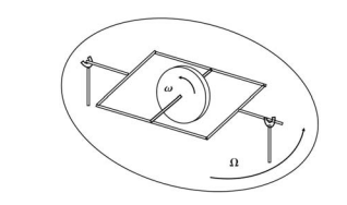
Gyroscopes Considerable simplification and practical application results if the angular velocity ω is an order of magnitude larger than angular velocity associated with the motions of a system of interest, such as an aircraft or a  spacecraft. In this case, the gyroscope can be used as an instrument to measure some quantity of interest in a vehicle. In order to use a gyroscope as an instrument, we first have to consider how it is mounted and affixed to the vehicle. The classic mount is called a gimbal. It permits free rotation of the gyroscope about its own axis, and depending on how complex the gimbal system is, free rotation about other axis as well.

Consider the gyroscope shown in the figure. It is free to spin about its axis with angular velocity ω. It is attached to a gimbal which is free to rotate about the support as sketched. The entire apparatus is mounted on a turntable rotating with angular velocity Ω, where ω >> Ω. If we can measure the orientation of the axis of rotation of the disk relative to the turntable mount, we could possibly use this as an instrument. What does it measure? Consider that the initial angular momentum vector of the disk is in the horizontal plane. The axis of the disk is free to rotate about the horizontal axis through an angle θ. As the turntable rotates with angular velocity Ω, the axis of the disk will rotate in θ–its only free direction– to keep its rate of change of angular momentum zero, since it can experience no moments/torques. There are two sources of changes in angular momentum, the unsteady component if θ changes with time; and the component of the angular momentum of the disk in the horizontal plane that is precessed by the turntable rotation Ω.

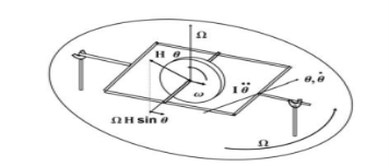
The unsteady ¨ term is I0θ, where I0 is the moment of inertia of the disk about the axis perpendicular to its spin axis; the vector is in the horizontal direction. The horizontal component of the angular momentum of the disk is Iωsinθ, where I is the moment of inertia of the disk about its axis of rotation. The rate of change is also in the horizontal direction, perpendicular to Ω and of magnitude IωΩsinθ. The sum of these two terms, which must be zero, is ¨

I0θ + IωΩsinθ = 0 this is the familiar equation for the oscillation of a pendulum. If there is a small amount of friction in the support, the system will settle at θ = 0 and will indicate the direction of rotation of the turntable axis. This is perhaps not too interesting, since we already know the direction of rotation of the turntable. But if we have this device on a rotating body, such as the earth, it will again indicate the direction of the axis of rotation of the body, in this case the earth. We call this direction “North”. Thus, this application of the gyroscope could be used as a compass, often called a gyrocompass.

Free precession

For round objects rolling on or in another round object, the analysis is similar to that for rolling on a at surface. A common application is the so-called epicyclic, hypo-cyclic, or planetary gears on planetary gears. Referring to F we can calculate the velocity of C with respect to a fixed frame two ways and Compare

Example: Two quarters.

The formula above can be tested in the case of R1 D R2 by using two quarters or

Two dimes on a table. Roll one quarter; call it B, around another quarter pressed

Fast to the table. You will see that as the rolling quarter B travels around the Stationary quarter one time, it makes two full revolutions. That is, the orientation

Of B changes twice as fast as the angle of the line from the Center of the stationary

Quarter to its centre. Or, in the language of the calculation

6.4 Rolling coin:

Roll ing coin

To solve the problem of a precessing rolling coin, you need a co-ordinate system

Which lends itself to circular movements. Intrinsic co-ordinates does this well.

An overview of intrinsic co-ordinates

The variable s is defined as the distance along the curve from some fixed point on the

Curve. The angle   is the angle made by the tangent to the curve at some variable

Point with the positive direction of the x-axis, see Figure 1

Roll ing coin

To solve the problem of a precessing rolling coin, you need a co-ordinate system

Which lends itself to circular movements. Intrinsic co-ordinates does this well.

An overview of intrinsic co-ordinates

The variable s is defined as the distance along the curve from some fixed point on the

Curve. The angle   is the angle made by the tangent to the curve at some variable

Point with the positive direction of the x-axis, see Figure 1

Rolling coin

To solve the problem of a precessing rolling coin, you need a co-ordinate system which lends itself to circular movements. Intrinsic co-ordinates does this well.

An overview of intrinsic co-ordinates

The variable s is defined as the distance along the curve from some fixed point on the curve. The angle   is the angle made by the tangent to the curve at some variable point with the positive direction of the x-axis, see Figure 1

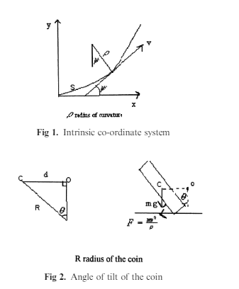
At some variable point on the curve the rate of change of s with respect to   is

Called the radius of curvat ure ! ¼ ds=d . Intrinsic co-ordinates are covered in detail

In the London ‘A’ Level Mathematics course. For further information on this co-

Ordinate frame please see my references

1;2

.

A coin rolled at a slight angle " to the vertical, see Figure 2, precesses like a

Gyroscope or a spinning top, with its axis free to move. So the precessional motion is

Combined with linear motion, see Figure 3, to produce a curved path.

The frictio nal force is F ¼ Mv

2

=!, this is necessary if the coin is to follow a curved

Path. From Figure 2 you can see the change in angular momentum (L) is due to the

Moment about

~

Oo. This moment acts to change the direction of the angular momentum

Of the coin, but not its magnitude. It is mathematically clear why this is so if you think

About the vector cross product.

Taking moments about

~

Oo : FR cos " " Mgd:

This is the change in angular momentum due to the moment about

~

Oo.

The tangent to the path makes an angle of   with the x-axis. So the change in the

Angular momentum in the x direction, as a result of a small rotation d  in tim e dt is

DL cos " ¼ L cos "d

At some variable point on the curve the rate of change of s with respect to ψ is

Called the radius of curvature w = ds /dψ

A coin rolled at a slight angle θ to the vertical, see Figure 2, processes like a gyroscope or a spinning top, with its axis free to move. So the processional motion is combined with linear motion, see Figure 3, to produce a curved path.

The frictional force is F= Mv2/w

This is necessary if the coin is to follow a curved path. From Figure 2 you can see the change in angular momentum (L) is due to the moment about

This moment acts to change the direction of the angular momentum of the coin, but not its magnitude. It is mathematically clear why this is so if you think about the vector cross product.

Taking moments about

= FR cosθ - Mgd

This is the change in angular momentum due to the moment about The tangent to the path makes an angle of ψ with the x-axis. So the change in the angular momentum in the x direction, as a result of a small rotation dψ in time dt is dL cosθ=L cosθ d

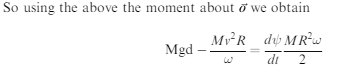
FR cosθ - Mgd = - dL/dt cos θ = - dψ / dt L.cosθ

Assuming that the coin is tilted only slightly we can use small angle approximations

Cos " # 1 and sin " ¼ d=R

Assuming that the coin is tilted only slightly we can use small angle approximations cosθ ≈1 and sinθ =d/R

Figure 4

a) The angular momentum (L) of the rolling coin and the horizontal component of L.

(b) Vector triangle showing the change in the angular momentum in the x-y plane.

a) The angular momentum (L) of the rolling coin and the horizontal component of L.

(b) Vector triangle showing the change in the angular momentum in the x-y plane.

The angular momentum L, of a disc with moment of inertia of MR2 / 2 about the rotation axis passing through the centre of mass is L= MR2w/2.

dψ /dt  is the angular speed of precession, so from Figure 1 this gives v=w dψ / dt   to the fact that the coin is rolling we can also say that

v= Rw

Using (1) with the rolling relationship you can show that

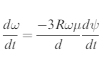
W=3Rv2/2gd

Then by differentiating above w.r.t. t obtain

Let k ¼ 3R#=d to simplify the algebra, then integrate equation (3) to obtain the

Radius of curvature at any point on the path a

Let k= 3 R μ /d to simplify the algebra, then integrate equation (3) to obtain the

Radius of curvature at any point on the path a

From these equations it can be seen that as the coin slows down, the rate of precession

Increases and the radius of curvature decreases

From these equations it can be seen that as the coin slows down, the rate of precession increases and the radius of curvature decreases.

UNIT 6

GENERAL MOTION

UNIT 6

GENERAL MOTION

UNIT 6

GENERAL MOTION

UNIT 6

GENERAL MOTION

6.1 General Planar motion

General plane motion of a rigid body refers to a combination of translation and rotation motion.

General planar motion refers to the simultaneous rotational and translational motion of a planar body in a 2-D plane.

General planar motion can be fully specified by knowing both the angular rotation of a line fixed in the body and the motion of any point on the body.

These motions can be related by using a rectilinear position coordinate s to locate the point along its path and an angular position coordinate to specify the orientation of the line. Then these two coordinates are related using the geometry of the problem. The following relation is found.

Differentiating the above equation, gives the relation between velocity and angular velocity .

Where,

Then again differentiating, it yields to the relation between acceleration and angular acceleration

Where,

Application: General Plane Motion

With the case of planar fixed axis rotation dealt with, we turn now to the more complex situation of general plane motion. Recall, once again, that the motion of an arbitrary rigid body can be reduced to the superposition of a translation and a fixed axis rotation. Handling the translation of a rigid body is trivial, all points of the body move with the same velocity and acceleration, and we now know how to deal with fixed axis rotations. Therefore, all that remains is to understand how the two are superposed. As we will find out, this is quite simple.

We proceed by returning to the equations we had derived for the arbitrary motion of a rigid body. Recall that these related the velocity  and acceleration  of a point A in the body to the translational motion of an arbitrary reference point B ( and ), and the absolute rotational motion of the body ( and ) as,

As in the case of fixed axis rotation we simplify these expressions by introducing a set of n-t coordinates. Unlike those used previously, however, the coordinates introduced here refer to the motion of A relative to the reference at B. Therefore,  is directed towards point B, the center of the relative motion, and  is directed along , tangent to the path of A relative to B.

Figure: n-t coordinates for general plane motion.

Substituting, we obtain a simplified expression for the velocity of point A,

Which can be recognized as a superposition of translational and rotational components, each of which we understand very well.

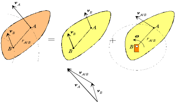
Figure : Decomposition of the absolute velocity of point A.

Proceeding in an analogous way for the acceleration,

Or,

With normal and tangential accelerations of the form,

Therefore, like the velocity, the acceleration of A is a superposition of translational and rotational components. While the normal component is directed along , towards the axis of the rotational motion of A relative to B, the tangential component is directed along , tangent to the path of A relative to B.

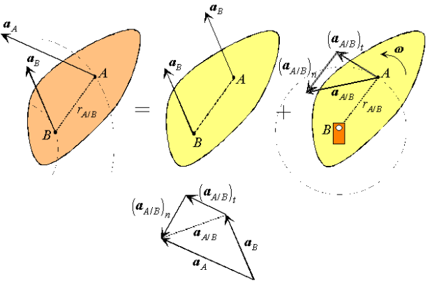
Figure : Decomposition of the absolute acceleration of point A.

For the general plane motion of a rigid body:

Alternately,

Where  is the position vector of A relative to the reference at B, ,  are the velocity and acceleration of the reference and ,  are the angular velocity and acceleration of the body.

6.2 Free or steady precession

Steady Precession: Gyroscopic Motion We now consider the steady precession of a top about the Z axis. In terms of the variables we have defined, the top rotates with spin velocity ψ˙ about its principal axis, and precesses with angular velocity φ˙ while maintaining a constant angle θ with the vertical axis Z. We then have

φ˙ = constant = φ˙ 0 φ¨ = 0

θ = constant = θ0 θ ˙ = ¨θ = 0

ψ˙ = 0 ψ¨ = 0

For a steady precession of a top, Euler’s equations reduce to

Φ sinθ (I(φ cos θ ˙ + ψ˙) − I0φcosθ) = Mx = MgsinθzG

Note that sinθ cancels, resulting in

Iφψ˙ − (I0 − I) φ˙2cosθ = MgzG

In the usual case for tops or gyroscopes, we have ψ >> φ˙ so that φ˙2 may be ignored. Therefore, for steady precession, the relationship between the precession angular velocity and the spin angular velocity is

φ˙ = MgzG/(Iψ˙)

Where I = Izz, the moment of inertia of the gyroscope about its spin axis. This result is also true if θ = 0. For this motion, the angular momentum vector is not aligned with the Z axis as for free-body motion, but is in the plane of z, Z, and rotates around the Z axis according to the applied external moment which is constant and in the x direction. In the limit as ψ˙ >> φ the angular momentum vector is essentially along the axis of ˙ rotation, z, with a slight component due to φ˙ which can be calculated after ψ˙ has been determined. Some attempt to sketch this is shown in the figure, but even this small correction is an approximation for ψ˙ >> φ.˙ F ˙ or ψ >> φ˙,

This same result can be obtained by less complex approach, but it is important to realize that this is an approximation. For the spin velocity much greater than the precessional velocity, we may take the angular momentum vector as directed along the spin or z axis,

H = Iω k. Then the applied moment will process the vector with rotation rate

Ω × H. Since Ω = ΩK = φK, (where K is a unit vector in the Z direction), this give a result for Ω in agreement with the previous result

Ω = MgzG/(Iω

Since θ dropped out of the previous equation, for θ = 0, we again have

Ω = MgzG/(Iω). The limit ψ˙ >> φ is the ”gyroscopic” limit where the device behaves as a gyroscope rather than as the more ˙ general case of a top. The difference is that, for a gyroscope, ω is larger than any other rotation rate in the system, such as the angular velocity of an aircraft or spacecraft. This makes the gyroscope a useful basis for many instruments.

6.3 Gyroscopes:

Gyroscopes Considerable simplification and practical application results if the angular velocity ω is an order of magnitude larger than angular velocity associated with the motions of a system of interest, such as an aircraft or a  spacecraft. In this case, the gyroscope can be used as an instrument to measure some quantity of interest in a vehicle. In order to use a gyroscope as an instrument, we first have to consider how it is mounted and affixed to the vehicle. The classic mount is called a gimbal. It permits free rotation of the gyroscope about its own axis, and depending on how complex the gimbal system is, free rotation about other axis as well.

Consider the gyroscope shown in the figure. It is free to spin about its axis with angular velocity ω. It is attached to a gimbal which is free to rotate about the support as sketched. The entire apparatus is mounted on a turntable rotating with angular velocity Ω, where ω >> Ω. If we can measure the orientation of the axis of rotation of the disk relative to the turntable mount, we could possibly use this as an instrument. What does it measure? Consider that the initial angular momentum vector of the disk is in the horizontal plane. The axis of the disk is free to rotate about the horizontal axis through an angle θ. As the turntable rotates with angular velocity Ω, the axis of the disk will rotate in θ–its only free direction– to keep its rate of change of angular momentum zero, since it can experience no moments/torques. There are two sources of changes in angular momentum, the unsteady component if θ changes with time; and the component of the angular momentum of the disk in the horizontal plane that is precessed by the turntable rotation Ω.

The unsteady ¨ term is I0θ, where I0 is the moment of inertia of the disk about the axis perpendicular to its spin axis; the vector is in the horizontal direction. The horizontal component of the angular momentum of the disk is Iωsinθ, where I is the moment of inertia of the disk about its axis of rotation. The rate of change is also in the horizontal direction, perpendicular to Ω and of magnitude IωΩsinθ. The sum of these two terms, which must be zero, is ¨

I0θ + IωΩsinθ = 0 this is the familiar equation for the oscillation of a pendulum. If there is a small amount of friction in the support, the system will settle at θ = 0 and will indicate the direction of rotation of the turntable axis. This is perhaps not too interesting, since we already know the direction of rotation of the turntable. But if we have this device on a rotating body, such as the earth, it will again indicate the direction of the axis of rotation of the body, in this case the earth. We call this direction “North”. Thus, this application of the gyroscope could be used as a compass, often called a gyrocompass.

Free precession

For round objects rolling on or in another round object, the analysis is similar to that for rolling on a at surface. A common application is the so-called epicyclic, hypo-cyclic, or planetary gears on planetary gears. Referring to F we can calculate the velocity of C with respect to a fixed frame two ways and Compare

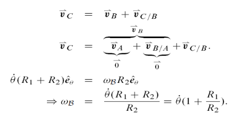
Example: Two quarters.

The formula above can be tested in the case of R1 D R2 by using two quarters or

Two dimes on a table. Roll one quarter; call it B, around another quarter pressed

Fast to the table. You will see that as the rolling quarter B travels around the Stationary quarter one time, it makes two full revolutions. That is, the orientation

Of B changes twice as fast as the angle of the line from the Center of the stationary

Quarter to its centre. Or, in the language of the calculation

6.4 Rolling coin:

Roll ing coin

To solve the problem of a precessing rolling coin, you need a co-ordinate system

Which lends itself to circular movements. Intrinsic co-ordinates does this well.

An overview of intrinsic co-ordinates

The variable s is defined as the distance along the curve from some fixed point on the

Curve. The angle   is the angle made by the tangent to the curve at some variable

Point with the positive direction of the x-axis, see Figure 1

Roll ing coin

To solve the problem of a precessing rolling coin, you need a co-ordinate system

Which lends itself to circular movements. Intrinsic co-ordinates does this well.

An overview of intrinsic co-ordinates

The variable s is defined as the distance along the curve from some fixed point on the

Curve. The angle   is the angle made by the tangent to the curve at some variable

Point with the positive direction of the x-axis, see Figure 1

Rolling coin

To solve the problem of a precessing rolling coin, you need a co-ordinate system which lends itself to circular movements. Intrinsic co-ordinates does this well.

An overview of intrinsic co-ordinates

The variable s is defined as the distance along the curve from some fixed point on the curve. The angle   is the angle made by the tangent to the curve at some variable point with the positive direction of the x-axis, see Figure 1

At some variable point on the curve the rate of change of s with respect to   is

Called the radius of curvat ure ! ¼ ds=d . Intrinsic co-ordinates are covered in detail

In the London ‘A’ Level Mathematics course. For further information on this co-

Ordinate frame please see my references

1;2

.

A coin rolled at a slight angle " to the vertical, see Figure 2, precesses like a

Gyroscope or a spinning top, with its axis free to move. So the precessional motion is

Combined with linear motion, see Figure 3, to produce a curved path.

The frictio nal force is F ¼ Mv

2

=!, this is necessary if the coin is to follow a curved

Path. From Figure 2 you can see the change in angular momentum (L) is due to the

Moment about

~

Oo. This moment acts to change the direction of the angular momentum

Of the coin, but not its magnitude. It is mathematically clear why this is so if you think

About the vector cross product.

Taking moments about

~

Oo : FR cos " " Mgd:

This is the change in angular momentum due to the moment about

~

Oo.

The tangent to the path makes an angle of   with the x-axis. So the change in the

Angular momentum in the x direction, as a result of a small rotation d  in tim e dt is

DL cos " ¼ L cos "d

At some variable point on the curve the rate of change of s with respect to ψ is

Called the radius of curvature w = ds /dψ

A coin rolled at a slight angle θ to the vertical, see Figure 2, processes like a gyroscope or a spinning top, with its axis free to move. So the processional motion is combined with linear motion, see Figure 3, to produce a curved path.

The frictional force is F= Mv2/w

This is necessary if the coin is to follow a curved path. From Figure 2 you can see the change in angular momentum (L) is due to the moment about

This moment acts to change the direction of the angular momentum of the coin, but not its magnitude. It is mathematically clear why this is so if you think about the vector cross product.

Taking moments about

= FR cosθ - Mgd

This is the change in angular momentum due to the moment about The tangent to the path makes an angle of ψ with the x-axis. So the change in the angular momentum in the x direction, as a result of a small rotation dψ in time dt is dL cosθ=L cosθ d

FR cosθ - Mgd = - dL/dt cos θ = - dψ / dt L.cosθ

Assuming that the coin is tilted only slightly we can use small angle approximations

Cos " # 1 and sin " ¼ d=R

Assuming that the coin is tilted only slightly we can use small angle approximations cosθ ≈1 and sinθ =d/R

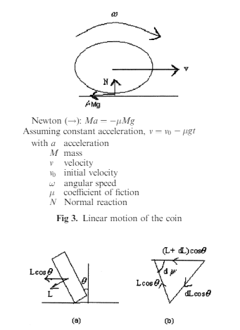
Figure 4

a) The angular momentum (L) of the rolling coin and the horizontal component of L.

(b) Vector triangle showing the change in the angular momentum in the x-y plane.

a) The angular momentum (L) of the rolling coin and the horizontal component of L.

(b) Vector triangle showing the change in the angular momentum in the x-y plane.

The angular momentum L, of a disc with moment of inertia of MR2 / 2 about the rotation axis passing through the centre of mass is L= MR2w/2.

dψ /dt  is the angular speed of precession, so from Figure 1 this gives v=w dψ / dt   to the fact that the coin is rolling we can also say that

v= Rw

Using (1) with the rolling relationship you can show that

W=3Rv2/2gd

Then by differentiating above w.r.t. t obtain

Let k ¼ 3R#=d to simplify the algebra, then integrate equation (3) to obtain the

Radius of curvature at any point on the path a

Let k= 3 R μ /d to simplify the algebra, then integrate equation (3) to obtain the

Radius of curvature at any point on the path a

From these equations it can be seen that as the coin slows down, the rate of precession

Increases and the radius of curvature decreases

From these equations it can be seen that as the coin slows down, the rate of precession increases and the radius of curvature decreases.