Unit-4

Sampling and Reconstruction

4.1 Sampling theorem and its implications

Sampling theorem states that “The continues form of a time-variant signal can be represented in the discrete form of a signal with help of samples and the sampled can be recovered to original form when the sampling signal frequency Fs having the greater frequency value than or equal to twice the input signal frequency Fm.

 Fs ≥ 2Fm

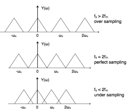
If the sampling frequency (Fs) equals twice the input signal frequency (Fm), then such a condition is called the Nyquist Criteria. When sampling frequency equals twice the input signal frequency is known as “Nyquist rate”.

Fs=2Fm

If the sampling frequency (Fs) is less than twice the input signal frequency, such criteria called an Aliasing effect.

Fs<2Fm

4.1.1 Spectra of sampled signals

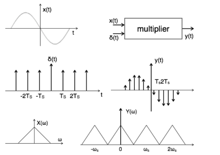
Consider a continuous time signal x(t). The spectrum of x(t) is a band limited to fm Hz that is the spectrum of x(t) is zero for |ω|>ωm.

Sampling of input signal x(t) can be obtained by multiplying x(t) with an impulse train δ(t) of period Ts. The output of multiplier is a discrete signal called sampled signal which is represented with y(t) in the following diagrams:

Figure1. Spectrum of the sampled signal

The sampled signal y(t) = x(t) . δ(t) ---------------------------------(1)

The Fourier series representation of δ(t) is given by

Taking Fourier transform on both the sides we get

Y(w) = 1/Ts [ X(w) + X(w-ws) + X(w+ws) + X(w-2ws) + X(w+2ws) +…..]

Y(w) = 1/Ts (w-nws) where n = 0, 1, …………

Figure 2. Sampled spectrum with different conditions

Key Take Aways:

The sampling theorem specifies the minimum-sampling rate at which a continuous-time signal needs to be uniformly sampled so that the original signal can be completely recovered or reconstructed by these samples alone

4.1.2 Reconstruction

4.1.2.1 Ideal Interpolator

The reconstructed analog signal involves weighing each individual discrete sample by a sinc function shifted-in-time by the sampling period. The sinc function:

P (t) = sin (π/Ts (t-nTs)]/ π/Ts (t-nTs) -------------------------------------------- (1)

is known as the ideal interpolation filter expressed in the frequency domain as:

P (F) = {1                 |F| < Fs/2

               0                 |F|   Fs/2 --------------------------------------------------(2)  

Applying the ideal interpolation filter in eel(2) to the spectrum of a non-aliased discrete-time signal results in recovering the original analog signal without any loss of information, as shown in Figure .

Figure 3. Recovered sampled spectrum of original analog signal.

To start with filtering the spectrum of the discrete-time signal by the interpolation filter eel (2), that is:

(F/Fs) = X(F/Fs) P(F)-----------------------------------------------------------(3)

Multiplication in the frequency domain is convolution in the time domain,

4.1.2.2 Zero Order Hold

The continuous - time signal is multiplied with a periodic impulse train, referred to as Sampling Function. A sampled signal is then obtained as shown in figure below.

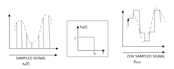
Figure 4. Sampled Zero Order Hold

p(t) = (t-nts) -------------------------------(1)

The ideally sampled signal up (t) is the product of the impulse train p (t) and the analog signal XC (t) which is written as

The ZOH Sampled Signal xZOH (t) can be regarded as the convolution of ho(t) and a sampled signal xp(t)

xzoH(t) = ho(t) * xp(t)-------------------------------------(5)

= ho(t) * [  δ(t-nts)]

= ho(t-nts)-----------------------------------------(6)

4.1.2.3 First Order Hold

Consider the signal

h1(t) =   1 - |t|/Ts        0 |t|<Ts

0                                               otherwise

A continuous signal x1(t) can be recovered by

x 1(t) can be recovered by

x1(t) = h1(t) * xs(t)

which is the linear interpolation of the sample train x(mTs) . This interpolation corresponds a low pass filtering in frequency domain by

H1(w) = F[h1(t)] = 4/w2 Ts sin2 (wsT/2)

Figure 5. First Order Hold

Key Take Aways:

The reconstruction process consists of replacing each sample by a sinc function, centered at the time of the sample and scaled by the sample value x(nT) times 2fc/ fs and adding all the functions so created

4.1.2.4 Aliasing and its effects

When the signal is converted back into a continuous time signal, it will exhibit a phenomenon called aliasing.  Aliasing is the presence of unwanted components in the reconstructed signal.  These components were not present when the original signal was sampled. 

In addition, some of the frequencies in the original signal may be lost in the reconstructed signal.  Aliasing occurs because signal frequencies can overlap if the sampling frequency is too low.  Frequencies "fold" around half the sampling frequency - which is why this frequency is often referred to as the folding frequency.

Key Take Aways:

Aliasing occurs when a signal is sampled at a less than twice the highest frequency present in the signal

4.2 Relation between continuous and discrete systems

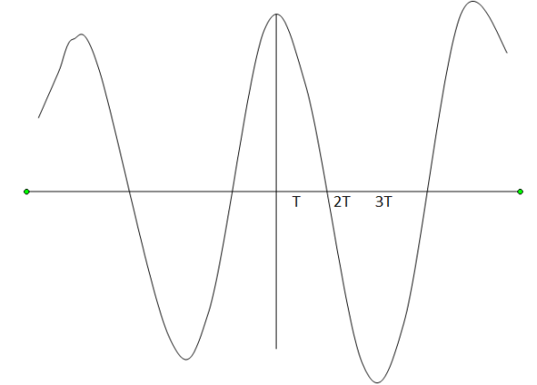
Let's start sampling a continuous-time signal, as shown in this graph:

Figure 6. Sampled signal

Mathematically, the relationship between the discrete-time signal and the continuous-time signal is given by:

x[n] = xc(nT) -------------------------------------------(1)

The sampling frequency is   fs = 1/T  (in Hz) orΩs= 2π/T  (in radians per second).

The discrete-time Fourier transform of x[n] is related to the continuous-time Fourier transform of xc(t) as follows:

X(w) = 1/T (w/T +2πk/T)

There are two key pieces to this equation.

The first is a scaling relationship between w and Ω : w=ΩT . This means that the sampling frequency in the continuous-time Fourier transform, Ωs , becomes the frequency 2π in the discrete-time Fourier transform.

The discrete-time frequency w=π corresponds to half the sampling frequency, or Ωs/2 .

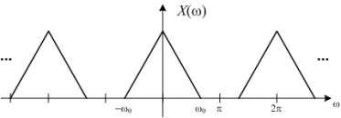
The second key piece of the equation is that there are an infinite number of copies of Xc(w/T) spaced by 2π .

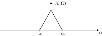
 Suppose Xc(Ω )looks like this:

Figure 7. Spectrum Xc(Ω)

Note that Xc(Ω)  equals zero for all frequencies |Ω| >Ωo . This means the continuous-time signal is band-limited. The frequency Ωo is called the bandwidth of the signal.

The discrete-time Fourier transform of xc=x[nT]  looks like this:

Figure 8. Discrete spectrum

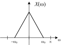
where wo=ΩoT . One period of X(w) is shown:

Figure 9. Scaled version

For this example, then, X(w) between -π and π looks just like a scaled version of Xc(Ω) .

Key Take Aways:

If a continuous time signal  x(t)   that has been sampled each  T    seconds to produce a discrete time signal  x(n) .

4.3 Introduction to the application of Signal And System Theory

4.3.1 Modulation for communication

A message carrying signal has to be transmitted over a distance and to establish a reliable communication, it needs to take the help of a high frequency signal which should not affect the original characteristics of the message signal.

The characteristics of the message signal, if changed, the message contained in it also alters. Hence care must be taken of the message signal. A high frequency signal can travel up to a longer distance, without getting affected by external disturbances.

We take the help of such high frequency signal which is called as a carrier signal to transmit our message signal. Such a process is simply called as Modulation.

Modulation is the process of changing the parameters of the carrier signal, in accordance with the instantaneous values of the modulating signal.

4.3.2 Filtering

The concept of filtering is a direct consequence of the fact that for linear, time-invariant systems the Fourier transform of the output is the Fourier transform of the input multiplied by the frequency response, that is the Fourier transform of the impulse response.

Because of this, the frequency content of the output is the frequency content of the input shaped by this frequency response. Frequency-selective filters attempt to exactly pass some bands of frequencies and exactly reject others. Frequency-shaping filters more generally attempt to reshape the signal spectrum by multiplying the input spectrum by some specified shaping.

Ideal frequency-selective filters, such as lowpass, highpass, and bandpass filters, are useful abstractions mathematically but are not exactly implementable.

4.3.3 Feedback Control Systems

A feedback control system is a system whose output is controlled using its measurement as a feedback signal. This feedback signal is compared with a reference signal to generate an error signal which is filtered by a controller to produce the system's control input. The block diagram below illustrates a general feedback system.

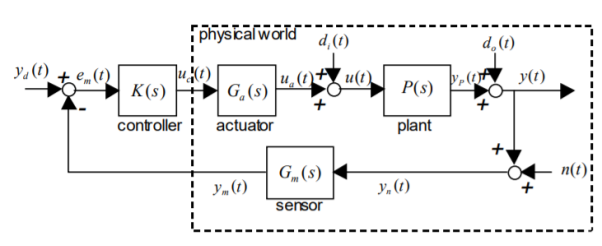
Figure. Feedback system

The controlled system is called the plant, and its LTI model is the transfer function P (s ). The disturbed output of the plant is y (t) and its noisy measurement is my(t ) corrupted by the measurement noise n (t ) . The error between the desired output dy(t ) (or reference) and my(t ) is the measured error, denoted as me(t ) . The output disturbance is the signal d(to )  and the output measurement noise is n(t ) .

The feedback measurement sensor dynamics are modelled by Gs(m ). The actuator (e.g., a valve) modelled by G (s ) is the device that translates a control signal from the controller K (s ) into an action on the plant input. The input disturbance signal d(ti ) disturbs the control signal from the actuator to the plant input.                                         

Key Take Aways:

Signals and Systems covers analog and digital signal processing, ideas at the heart of modern communication and measurement. 

References:

     Signals and Systems by Simon Haykin

     Signals and Systems by Ganesh Rao

     Signals and Systems by P. Ramesh Babu

     Signals and Systems by Chitode