Unit 2
Time Response Analysis
Unlike electric networks and communication systems, the inputs to many practical control systems are not exactly known ahead of time. In many cases, the actual inputs of a control system may vary in random fashion with respect to time. For instance, in a radar-tracking system for antiaircraft missiles, the position and speed of the target to be tracked may vary in an unpredictable manner, so that they cannot be predetermined. This poses a problem for the designer, because it is difficult to design a control system so that it will perform satisfactorily to all possible forms of input signals.
For the purpose of analysis and design, it is necessary to assume some basic types of test inputs so that the performance of a system can be evaluated. By selecting these basic test signals properly, not only is the mathematical treatment of the problem systematized, but the response due to these inputs allows the prediction of the system’s performance to othermore complex inputs.
In the design problem, performance criteria may be specified withrespect to these test signals so thatthe system may be designed to meet the criteria. This approach is particularly useful forlinear systems, since the response to complex signals can be determined by superposing those due to simple test signals. When the response of a linear time-invariant systemis analyzed in the frequency domain, a sinusoidal input with variable frequency is used. When the input frequency is swept from zero to beyond the significant range of the system characteristics, curves in terms of the amplitude ratio and phasebetween the input and the output are drawn as functions of frequency. It is possible to predict the time-domain behavior of the system from its frequency-domain characteristics.
To facilitate the time-domain analysis, the following deterministic test signals are used.
a) Step-Function Input:
The step-function input represents an instantaneous change in the reference input. For example, if the input is an angular position of a mechanical shaft, a step input represents the sudden rotation of the shaft. The mathematical representation of a step function or magnitude R is


Where R is a real constant. Or

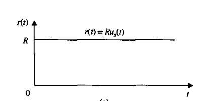
Where us(t) is the unit-step function. The step function as a function of time is shown in above figure. The step function is very useful as a test signal because its initial instantaneous jump in amplitude reveals a great deal about a system's quickness in responding to inputs with abrupt changes. Also, because the step function contains, in principle, a wide band of frequencies in its spectrum, as a result of the jump discontinuity, it is equivalent to the application of numerous sinusoidal signals with a wide range of frequencies.
b) Ramp-Function Input:
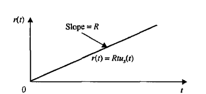
The ramp function is a signal that changes constantly with time. Mathematically, a ramp function is represented by

Where R is a real constant. The ramp function is shown in Figure below. If the input variable represents the angular displacement of a shaft, the ramp input denotes the constant-speed rotation of the shaft. The ramp function has the ability to test how the system would respond to a signal that changes linearly with time.
c) Parabolic-Function Input:
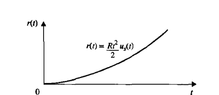
The parabolic function represents a signal that is one order faster than the ramp function. Mathematically, it is represented as

Where R is a real constant and the factor 1/2, is added for mathematical convenience because the Laplace transform of r(t) is simply R/s3. The graphical representation of the parabolic function is shown in figure below.
If the output of control system for an input varies with respect to time, then it is called the time response of the control system. The time response consists of two parts.
a) Transient response
b) Steady state response
The response of control system in time domain is shown in the following figure.
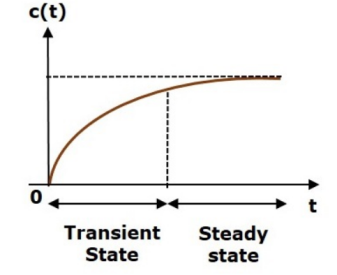
Here, both the transient and the steady states are indicated in the figure. The responses corresponding to these states are known as transient and steady state responses.
Mathematically, we can write the time response c(t) as

Where, ctr(t) is the transient response and css(t) is the steady state response
Transient Response
After applying input to the control system, output takes certain time to reach steady state. So, the output will be in transient state till it goes to a steady state. Therefore, the response of the control system during the transient state is known as transient response.
The transient response will be zero for large values of ‘t’. Ideally, this value of ‘t’ is infinity and practically, it is five times constant.
Mathematically, we can write it as
LimCtr(t)=0
t->∞
Steady state Response
The part of the time response that remains even after the transient response has zero value for large values of ‘t’ is known as steady state response. This means, the transient response will be zero even during the steady state.
Time response of first order system
Consider the following block diagram of the closed loop control system. Here, an open loop transfer function, 1/sT is connected with a unity negative feedback.

We know that the transfer function of the closed loop control system has unity negative feedback as

Substitute, 

The power of s is one in the denominator term. Hence, the above transfer function is of the first order and the system is said to be the first order system.
We can re-write the above equation as

Where,
C(s) is the Laplace transform of the output signal c(t).
R(s) is the Laplace transform of the input signal r(t) , and
T is the time constant
Follow these steps to get the response (output) of the first order system in the time domain
1. Take the Laplace transform of the input signal r(t)
2. Consider the equation,

3. Substitute R(s) value in the above equation
4. Do partial fractions of C(s)if required.
5. Apply inverse Laplace transform to C(s)
a) Impulse Response of First Order System
Consider the unit impulse signal as an input to the first order system

Apply Laplace transform on both the sides.

Substitute , R(s)=1 in the above equation

Rearrange the above equation in one of the standard forms of Laplace transforms.

Apply inverse Laplace transform on both sides

The unit impulse response is shown in the following figure
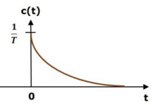
Th The unit impulse response, c(t) is an exponential decaying signal for positive values of ‘t’ and it is zero for negative values of ‘t’ i.eunit impulse response, c(t) is an exponential decaying signal for positive values of ‘t’ and it is zero for negative values of ‘t’.
b) Step Response of First Order System
Consider the unit step signal as an input to first order system.

Apply Laplace transform on both the sides.

Consider the equation ,  in the above equation

Do partial fractions of C(s)


On both the sides, the denominator term is the same. So, they will get cancelled by each other. Hence, equate the numerator terms.

By equating the constant terms on both the sides, you will get A = 1. Substitute, A = 1 and equate the coefficient of the s terms on both the sides.

Substitute, A=1 and B =-T in the partial fraction expansion of C(s)


Apply inverse Laplace transform on both the sides

The unit step response, c(t) has both the transient and the steady state terms.
The transient term in the unit step response is –

The steady state term in the unit step response is –

The following figure shows the unit step response.
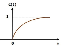
The value of the unit step response, c(t) is zero at t = 0 and for all negative values of t. It is gradually increasing from zero value and finally reaches to one in steady state. So, the steady state value depends on the magnitude of the input.
Initial value theorem and Final value theorem are together called as Limiting Theorems. Initial value theorem is often referred as IVT. It will enable us to find the initial value at time t = (0+) for a given transformed function (Laplace) without enabling us work harder to find f(t) which is a tedious process in such case.
Conditions for the existence of Initial value theorem
- The function f(t) and its derivative f(t) should be Laplace transformable.
- If time t approaches to (0+) then the function f(t) should exists.
{i.e. lim f(t) should exist }
t-> 0+
3. The function f(t) = 0 for t > 0 and contains no impulses or higher order singularities at origin.
Statement of Laplace Initial Value Theorem
If f(t) and F(s) is Laplace transform pairs. i.e.

Then Initial value theorem is given by

Applications of Initial Value Theorem
Purpose of initial value theorem is to determine the initial value of the function f (t) provided its Laplace transform is given
Example 1:
Find the initial value for the function f (t) = 2 u (t) + 3 cost u (t)


By initial value theorem

Here, 
Final value theorem
Final Value Theorem is used for determining the final value of a Laplace domain function F(s). Though we can always transform a time domain function into Laplace domain to apply Final Value Theorem. According to Final Value Theorem, final value of a function i.e. value of function f(t) when t→∞ is given as,
Final value of f(t)= lim sF(s)
s-> 0
However, whether a given function f(t) has a final value or not depends on the locations of the poles of its transform F(s). Consider the following cases:
- If there are poles on the right side of the S-plane, f(t) will contain exponentially growing terms and therefore is not bounded, f(∞) does not exist.
- If there are pairs of complex conjugate poles on the imaginary axis, f(t) will contain sinusoidal components and f(∞) is not defined.
- If there are poles on the left side of the S-plane, f(t) will contain exponentially decaying terms without contribution to the final value.
- Only when there are poles at the origin of the S-plane, f(t)will contain constant (DC) component which is the final value, the steady state of the signal.
Applications of Final Value Theorem
The final value theorem can also be used to find the DC gain of the system, the ratio between the output and input in steady state when all transient components have decayed. We assume the input is a unit step function f(t)=u(t), and find the final value, the steady state of the output, as the DC gain of the system.
Let us consider some examples to better understand the application of Final Value Theorem.
Example-2:
Find the steady state value of function given below
F(s) = 1/s(s+2)(s+5)
Solution:
Steady value of function means the final value. Hence for the above example, we will calculate final value.
Since, F(s) = 1/s(s+2)(s+5)
So, sF(s) = 1/(s+2)(s+5)
Using Final Value Theorem,
Final value =lim sF(s)
S-> 0
Lim{1/(s+2)(s+5)}
S->0
1/10=0.1 ans
Let us discuss the time domain specifications of the second order system. The step response of the second order system for the underdamped case is shown in the following figure.
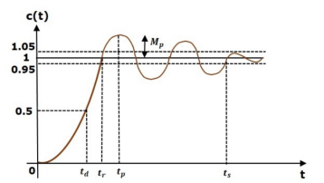
All the time domain specifications are represented in this figure. The response up to the settling time is known as transient response and the response after the settling time is known as steady state response.
Delay Time
It is the time required for the response to reach half of its final value from the zero instant. It is denoted by td. Consider the step response of the second order system for t ≥ 0, when ‘δ’ lies between zero and one.

The final value of the step response is one.
Therefore, at t=td , the value of the step response will be 0.5. Substitute, these values in the above equation.


By using linear approximation you will get the delay time 

Rise Time
It is the time required for the response to rise from 0% to 100% of its final value. This is applicable for the under-damped systems. For the over-damped systems, consider the duration from 10% to 90% of the final value. Rise time is denoted by tr.
At t = t1 = 0, c(t) = 0.
We know that the final value of the step response is one.
Therefore, at t=t2 , the value of step response is one. Substitute, these values in the following equation.


Substitute t1 and t2 values in the following equation of rise time.


From above equation, we can conclude that the rise time tr and the damped frequency ωd are inversely proportional to each other.
Peak Time
It is the time required for the response to reach the peak value for the first time. It is denoted by tp. At t=tp, the first derivate of the response is zero.
We know the step response of second order system for under-damped case is

Differentiate c(t) with respect to “t”

Substitute, 


From the above equation, we can conclude that the peak time tp and the damped frequency ωd are inversely proportional to each other.
Peak Overshoot
Peak overshoot Mp is defined as the deviation of the response at peak time from the final value of response. It is also called the maximum overshoot. Mathematically, we can write it as

Where, c(tp) is the peak value of the response. c(∞) is the final (steady state) value of the response. At t=tp, the response c(t) is –

Substitute 


We know that

So, we will get 

Substitute the values of 


By substituting the values of Mp and c(∞) in above formula, we will get the Percentage of the peak overshoot %Mp as

From the above equation, we can conclude that the percentage of peak overshoot %Mp will decrease if the damping ratio δincrease.
Settling time
It is the time required for the response to reach the steady state and stay within the specified tolerance bands around the final value. In general, the tolerance bands are 2% and 5%. The settling time is denoted by ts.
The settling time for 5% tolerance band is

The setting time for 2% tolerance band is-

Where ,
Both the settling time ts and the time constant τ are inversely proportional to the damping ratio δ.
Both the settling time ts and the time constant τ are independent of the system gain.
That means even the system gain changes, the settling time ts and time constant τ will never change.
A system is said to be stable, if its output is under control. Otherwise, it is said to be unstable. A stable system produces a bounded output for a given bounded input.
The following figure shows the response of a stable system
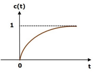
This is the response of first order control system for unit step input. This response has the values between 0 and 1. So, it is bounded output. We know that the unit step signal has the value of one for all positive values of t including zero. So, it is bounded input. Therefore, the first order control system is stable since both the input and the output are bounded.
Types of Systems based on Stability
We can classify the systems based on stability as follows.
- Absolutely stable system
- Conditionally stable system
- Marginally stable system
Absolutely Stable System
If the system is stable for all the range of system component values, then it is known as the absolutely stable system. The open loop control system is absolutely stable if all the poles of the open loop transfer function present in left half of ‘s’ plane. Similarly, the closed loop control system is absolutely stable if all the poles of the closed loop transfer function present in the left half of the ‘s’ plane.
Conditionally Stable System
If the system is stable for a certain range of system component values, then it is known as conditionally stable system.
Marginally Stable System
If the system is stable by producing an output signal with constant amplitude and constant frequency of oscillations for bounded input, then it is known as marginally stable system. The open loop control system is marginally stable if any two poles of the open loop transfer function is present on the imaginary axis. Similarly, the closed loop control system is marginally stable if any two poles of the closed loop transfer function is present on the imaginary axis.
Routh-Hurwitz stability criterion is having one necessary condition and one sufficient condition for stability.
If any control system doesn’t satisfy the necessary condition, then we can say that the control system is unstable. But, if the control system satisfies the necessary condition, then it may or may not be stable.
So, the sufficient condition is helpful for knowing whether the control system is stable or not.
Necessary Condition for Routh-Hurwitz Stability
The necessary condition is that the coefficients of the characteristic polynomial should be positive. This implies that all the roots of the characteristic equation should have negative real parts.
Consider the characteristic equation of the order ‘n’ is –

Note that, there should not be any term missing in the nth order characteristic equation. This means that the nth order characteristic equation should not have any coefficient that is of zero value.
Sufficient Condition for Routh-Hurwitz Stability
The sufficient condition is that all the elements of the first column of the Routh array should have the same sign.
This means that all the elements of the first column of the Routh array should be either positive or negative
Routh Array Method
If all the roots of the characteristic equation exist to the left half of the‘s’ plane, then the control system is stable.
If at least one root of the characteristic equation exists to the right half of the‘s’ plane, then the control system is unstable.
So, we have to find the roots of the characteristic equation to know whether the control system is stable or unstable. But, it is difficult to find the roots of the characteristic equation as order increases.
So, to overcome this problem there we have the Routh array method. In this method, there is no need to calculate the roots of the characteristic equation.
First formulate the Routh table and find the number of the sign changes in the first column of the Routh table. The number of sign changes in the first column of the Routh table gives the number of roots of characteristic equation that exist in the right half of the ‘s’ plane and the control system is unstable.
Follow this procedure for forming the Routh table.
a) Fill the first two rows of the Routh array with the coefficients of the characteristic polynomial as mentioned in the table below. Start with the coefficient of S and continue up to the coefficient of S0
b) Fill the remaining rows of the Routh array with the elements as mentioned in the table below. Continue this process till you get the first column element of row s0 is an. Here, an is the coefficient of s0 in the characteristic polynomial.
The following table shows the Routh array of the nth order characteristic polynomial

 |  |  |  |  | … | … |
 |  |  |  |  | … | … |
 |  |  |  | … | … | … |
 |  |  | : |
|
|
|
: | : | : | : |
|
|
|
 | : | : |
|
|
|
|
 |  |
|
|
|
|
|
The root locus is a graphical representation in s-domain and it is symmetrical about the real axis. Because the open loop poles and zeros exist in the s-domain having the values either as real or as complex conjugate pairs.
Rules for Construction of Root Locus
Follow these rules for constructing a root locus.
Rule 1− Locate the open loop poles and zeros in the ‘s’ plane.
Rule 2− Find the number of root locus branches.
We know that the root locus branches start at the open loop poles and end at open loop zeros. So, the number of root locus branches N is equal to the number of finite open loop poles P or the number of finite open loop zeros Z, whichever is greater.
Mathematically, we can write the number of root locus branches N as


Rule 3− Identify and draw the real axis root locus branches.
If the angle of the open loop transfer function at a point is an odd multiple of 1800, then that point is on the root locus. If odd number of the open loop poles and zeros exist to the left side of a point on the real axis, then that point is on the root locus branch. Therefore, the branch of points which satisfies this condition is the real axis of the root locus branch.
Rule 4− Find the centroid and the angle of asymptotes.
a) If P=Z then all the root locus branches start at finite open loop poles and end at finite open loop zeros.
b) If P>Z , then Z number of root locus branches start at finite open loop poles and end at finite open loop zeros and P−Z number of root locus branches start at finite open loop poles and end at infinite open loop zeros.
c) If P<Z , then P number of root locus branches start at finite open loop poles and end at finite open loop zeros and Z−P number of root locus branches start at infinite open loop poles and end at finite open loop zeros.
So, some of the root locus branches approach infinity, when P≠Z. Asymptotes give the direction of these root locus branches. The intersection point of asymptotes on the real axis is known as centroid. We can calculate the centroid α by using this formula

The formula for the angle of asymptotes  is
is

Where,
Q=0, 1, 2,…, (P-Z)-1
Rule 5− Find the intersection points of root locus branches with an imaginary axis.
We can calculate the point at which the root locus branch intersects the imaginary axis and the value of K at that point by using the Routh array method and special case (ii).
- If all elements of any row of the Routh array are zero, then the root locus branch intersects the imaginary axis and vice-versa.
- Identify the row in such a way that if we make the first element as zero, then the elements of the entire row are zero. Find the value of K for this combination.
- Substitute this K value in the auxiliary equation. You will get the intersection point of the root locus branch with an imaginary axis.
Rule 6− Find Break-away and Break-in points.
- If there exists a real axis root locus branch between two open loop poles, then there will be a break-away point in between these two open loop poles.
- If there exists a real axis root locus branch between two open loop zeros, then there will be a break-in point in between these two open loop zeros.
Note− Break-away and break-in points exist only on the real axis root locus branches.
Follow these steps to find break-away and break-in points.
a) Write K in terms of s from the characteristic equation 1+G(s)H(s)=0.
b) Differentiate K with respect to s and make it equal to zero.
Substitute these values of s in the above equation. The values of s for which the K value is positive are the break points.
Rule 7− Find the angle of departure and the angle of arrival.
The Angle of departure and the angle of arrival can be calculated at complex conjugate open loop poles and complex conjugate open loop zeros respectively.
The formula for the angle of departure  is
is

The formula for the angle of arrival  is
is

Where,
