Unit 5
State variable Analysis
In contrast to the transfer-function approach to the analysis and design of linear control systems, the state-variable method is regarded as modern, since it uses underlying force for optimal control. The basic characteristic of the state-variable formulation is that linear and nonlinear systems, time-invariant and time-varying systems, and single-variable and multivariable systems can all be modelled in a unified manner. Transfer functions, on the other hand, are defined only for linear time-invariant systems.
The process by which the state of a system is determined is called state variable analysis.
Advantages of State Space Techniques
- This technique can be used for linear or nonlinear, time-variant or time-invariant systems.
- It is easier to apply where Laplace transform cannot be applied.
- The nth order differential equation can be expressed as 'n' equation of first order.
- It is a time domain method.
- As this is time domain method, therefore this method is suitable for digital computer computation.
- On the basis of the given performance index, this system can be designed for an optimal condition.
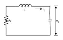
Consider an RLC network, At time t = 0, Current = iL (0), Capacitor Voltage = Vc (0)
Thus, the state of the network at time t=0 is specified by the inductor current and capacitor voltage. State Space representation of electrical system:
Therefore iL(0) and Vc(0) is called the initial state of the network and the pair iL(t), Vc(t) is called the state of the network at 't'. The variable iL and Vc are called the state variables of the network.

Apply KVL

Also

From eq. 1


This type of equation is called State equation. And the variables present in this equation are called state variables.
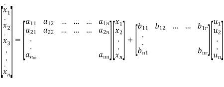
Eq. 3 and Eq. 4 can be written in matrix form as

Let 
The general form of state equation is


Y = n- dimensional output vector
U = r-dimensional control vector or input vector
A = n × n system matrix
B = n × r control matrix
C = n × n output matrix
When there is no direct connection between input and output in that case D u(t) is not taken.


State Space Representation of nth order differential Equation
For the nth order differential equation
To obtain the modal representation, we may diagonalize any state-space representation. This is accomplished by means of a particular similarity transformation specified by the eigenvectors of the state transition matrix . An eigenvector of the square matrix
  is any vector eifor which

Where λi may be complex. In other words, when the matrix  of the similarity transformation is composed of the eigenvectors of
  ,
,

The transformed system will be diagonalized, as we will see below.
A system can be diagonalized whenever the eigenvectors of  are linearly independent. This always holds when the system poles are distinct. It may or may not hold when poles are repeated.
To see how this works, suppose we are able to find  linearly independent eigenvectors of
  , denoted ei, i=1,2, ……, N, then we can form an NxN matrix
  having these eigenvectors as columns.
Since the eigenvectors are linearly independent,  is full rank and can be used as a one-to-one linear transformation, or change-of-coordinates matrix. We have that the transformed state transition matrix is given by


Which shows that the new state transition matrix is diagonal and made up of the eigenvalues of  .
.
Transfer function of single input and single out system is


We have incidentally shown that the eigenvalues of the state-transition matrix  are the poles of the system transfer function. When it is diagonal, i.e., when
 diag,
diag, the state-space model may be called a modal
Representation of the system, because the poles appear explicitly along the diagonal of  and the system's dynamic modes are decoupled.
The response of linear, time-invariant models expressed in the standardstate -equation form


That is, as a set of coupled, first-order differential equations. The solution proceeds in twosteps; first the state-variable response x(t) is found by solving the set of first-order state equations, Eq. (1), and then the state response is substituted into the algebraic output equations, Eq. (2) in order to compute y(t).
The Homogeneous State Response
The state-variable response of a system described by Eq. (1) with zero input, u(t)≡0, and an arbitrary set of initial conditions x (0) is the solution of the set of n homogeneous first-order differential equations
 =Ax
=Ax
To derive the homogeneous response xh(t), we begin by considering the response of a first-order (scalar) system with state equation

With initial condition x (0). In this case the homogeneous response xh(t) has an exponential form defined by the system time constant τ=−1/a, or

 ----------------6
 -------------7
Where x (0) is the initial state. Each term in this series is a matrix of size n×n, and the summation of all terms yields another matrix of size n×n. To verify that the homogeneous state equation ̇x=Axis satisfied by Eq. (7), the series may be differentiated term by term. Matrix differentiation is defined on an element by element basis, and because each system matrix Ak contains only constant elements


The homogeneousresponse to an arbitrary set of initial conditionsx (0) can therefore be expressed as aninfinitesum of time dependent matrix functions, involving only the system matrix A. Because of thesimilarity of this series to the power series defining the scalar exponential, it is convenientto define thematrix exponentialof a square matrixAas

The system homogeneous response xh(t) may therefore be written in terms of the matrix exponential

The solution is often written as

Where Φ(t)=eAt is defined to be the state transition matrix [1 – 5]. Equation (11) gives the response at any time t to an arbitrary set of initial conditions, thus computation of eAt at any t yields the values of all the state variables x(t) directly.
The roots of the characteristic equation are often referred to as the eigenvalues of the matrix A.
Some of the important properties of eigenvalues are given as follows.
1. If the coefficients of A are all real, then its eigenvalues are either real or in complex-conjugate pairs.
2. If λ1, λ2, λ3 • • •λn, are the eigenvalues of A, then

That is, the trace of A is the sum of all the eigenvalues of A.
3. If λi, i = 1,2, ..., n, is an eigenvalue of A, then it is an eigenvalue of A'.
4. If A is non-singular, with eigenvalues λi, i = 1,2, ..., n, then 1/ λi, i = 1,2, ..., n, i = 1, 2, ..., n, are the eigenvalues of A -I.
The concepts of controllability and observability play an important role in both theoretical and practical aspects of modern control. The conditions on controllability and observability essentially govern the existence of a solution to an optimal control problem. This seems to be the basic difference between optimal control theory and classical control theory.
In the classical control theory, the design techniques are dominated by trial-anderror methods so that given a set of design specifications the designer at the outset does not know if any solution exists. Optimal control theory, on the other band, has criteria for determining at the outset if the design solution exists for the system parameters and design objectives
Concept of controllability
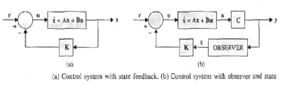
The concept of controllability can be stated with reference to the block diagram of following Fig (a).
The process is said to be completely controllable if every state variable of the process can be controlled to reach a certain objective infinite time by some unconstrained control u(t), as shown in Fig (b).
Intuitively, it is simple to understand that, if any one of the state variables is independent of the control u(t), there would be no way of driving this particular state variable to a desired state in finite time by means of a control effort.
Therefore, this particular state is said to be uncontrollable, and, as long as there is at least one uncontrollable state, the system is said to be not completely controllable or, simply, uncontrollable.
As a simple example of an uncontrollable system, Fig. 3 illustrates the state diagram of a linear system with two state variables. Because the control U(t) affects only the state x1(t), the state x2{t) is uncontrollable.
In other words, it would be impossible to drive x2(t) from an initial state x2(t0) to a desired state x2(t1) in finite time interval ti-t0 by the control U(t). Therefore, the entire system is said to be uncontrollable.
The concept of controllability given here refers to the states and is sometimes referred to as state controllability. Controllability can also be defined for the outputs of the system, so there is a difference between state controllability and output controllability


OBSERVABILITY OF LINEAR SYSTEMS
Essentially, a system is completely observable if every state variable of the system affects some of the outputs. In other words, it is often desirable to obtain information on the state variables from the measurements of the outputs and the inputs.
If any one of the states cannot be observed from the measurements of the outputs, the state is said to be unobservable, and the system is not completely observable or, simply. Unobservable.
Following figure shows the state diagram of a linear system in which the state x2 is not connected to the output y(t) in any way. Once we have measured y(t), we can observe the state x1(t), since x1(t) = y(t). However, the state x2 cannot be observed from the information on y(t). Thus, the system is unobservable.

When root loci are utilized for the design of control systems, the general approach may be described as that of pole placement; the poles here refer to that of the closed-loop transfer function, which are also the roots of the characteristic equation.
Knowing the relation between the closed-loop poles and the system performance, we can effectively carry out the design by specifying the location of these poles.
When we have a controlled process of the third order or higher, the PD, PI, single-stage phase-lead, and phase-lag controllers would not be able to control independently all the poles of the system, because there are only two free parameters in each of these controllers. To investigate the condition required for arbitrary pole placement in an nth-order system, let us consider that the process is described by the following state equation:

Where x(t) is an n x 1 state vector, and u(t) is the scalar control. The state-feedback control is

Where K is the 1 x n feedback matrix with constant-gain elements

|sI-A+BK| =0
The feedback gain matrix K is expressed as

Where  are real constant . Then,
The eigenvalues of A -BK are then found from the characteristic equation

Clearly, the eigenvalues can be arbitrarily assigned, because the feedback gains k1, k2, ••• kn are isolated in each coefficient of the characteristic equation.
Intuitively, it makes sense that a system must be controllable for the poles to be placed arbitrarily. If one or more state variables are uncontrollable, then the poles associated with these state variables are also uncontrollable and cannot be moved as desired.
Discrete time systems are either inherently discrete (e.g. Models of bank accounts, national economy growth models, population growth models, digital words) or they are obtained as a result of sampling (discretization) of continuous-time systems. In such kinds of systems, inputs, state space variables, and outputs have the discrete form and the system models can be represented in the form of transition tables.
The mathematical model of a discrete-time system can be written in terms of a recursive formula by using linear matrix difference equations as


Here represents the constant sampling interval, which may be omitted for brevity, that is, we use the following notation


Because digital controllers are frequently used in control systems, it is necessary to establish equations that relate digital and discrete-time signals. Just as differential equations are used to represent systems with analog signals, difference equations are used for computers or systems utilizing discrete data. Difference equations are also used to approximate differential equations, because the former is more easily programmed on a computer and are easier to solve. A linear nth-order difference equation with constant coefficients can be written as

Where y(i), i= k, k+1, …, k+n denotes the discrete dependent variable y at the ith instant if the independent variable is time.
In general, the independent variable can be any real quantity. Similar to the case of the analog systems, it is convenient to use a set of first-order difference equations, or state equations, to represent a high-order difference equation. For the above difference equation if we let


Then by equating the highest-order term to the rest, the equation is written as

The n state equations are written in vector-matrix form


Is nx1 state vector.

And u(k) =f(k)
State-space models describe a system’s dynamics via two equations:
•The “state equation” describes how the input influences the state;
•The “output equation” describes how the state and the input both directly influence the output.
Discrete-time LTI state-space models have the following form


Where u[k]∈Rm is the input, y[k]∈Rp is the output, and x[k]∈Rn is the state vector.
Different systems have different n, A, B, C and D.
The definitions of BIBO and zero-input stability can be readily extended to linear time-invariant SISO discrete-data control systems
BIBO Stability: Letu(kT),y(kT), andg(kT) be the input, output, and impulse sequence of a linear time-invariant SISO discrete-data system, respectively. Withzero initial conditions, the systemis said to be BIBO stable, or simply stable, if its output sequence y(kT)is bounded to abounded input u(kT). For the systems be BIBO stable, the following condition must be met:

Zero-Input Stability: For zero-input stability, the output sequence of the system must satisfy the following conditions
|y(KT)|<=M<∞
Lim |y(KT)=0
k->∞

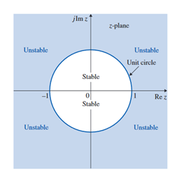
Stability condition | Root values |
Asymptotically stable or simply stable |  |
Marginally stable or marginally unstable |   |
Unstable |   |