Unit - 5
Applications of Digital Signal Processing
The power spectrum of a signal gives the distribution of the signal power among various frequencies. The power spectrum is the Fourier transform of the correlation function, and reveals information on the correlation structure of the signal. The strength of the Fourier transform in signal analysis and pattern recognition is its ability to reveal spectral structures that may be used to characterise a signal.
In general, the more correlated or predictable a signal, the more concentrated its power spectrum, and conversely the more random or unpredictable a signal, the more spread its power spectrum. Therefore, the power spectrum of a signal can be used to deduce the existence of repetitive structures or correlated patterns in the signal process. Such information is crucial in detection, decision making and estimation problems, and in systems analysis.
Definition of Correlation and Power Spectra
- Analog Random Signal
𝛄x y (τ) = E[x(t)y(t – τ)] = LimTp⟶∞ 1/ Tp ∫Tp/2– Tp/2 x(t)y(t – τ) dt
𝗿xy (F) = ∫∞-∞ 𝛄xy(τ)e-j2𝜋F𝜏 dτ
𝛄xy (τ) = ∫∞-∞ 𝗿xy (F)ej2𝜋F𝜏 dF
- Discrete time Random Signal
- 𝛄xy(m) = E[x(n)y(n-m)] = LimN⟶∞ 1/N ∑N-1n=0 x(n)y(n-m)
𝗿xy (𝒇) = ∑∞m=-∞ 𝛄xy (m)e-j2𝜋𝒇m
𝛄xy(m) = ∫1/2-1/2 𝗿xy(𝒇)ej2 𝜋𝒇m d𝒇
- Analog Periodic Signal
𝗿xp yp(τ) = 1/ Tp ∫Tp/2– Tp/2 xp(t)yp(t – τ) dt = xp(τ) * yp(-τ)
Sxp yp(k) = 1/ Tp ∫Tp/2– Tp/2 rxp yp(τ)e-j2𝜋 k/Tp τ dτ
𝗿xp yp(τ) = ∑∞k=-∞ Sxp yp(k) e-j2𝜋 k/Tp 𝜏
- Discrete time Periodic Signal


Properties of Autocorrelation Function
Random | Periodic | Aperiodic |
 |  |  |
 |  |  |
 |  |  |
 |  |  |
 |  |  |
Properties of Power Spectra
Random | Periodic | Aperiodic |
 |  |  |
  |   |  |
  |  |  |
Cont. Real. Spect+  | Real discrete spect at  | Const real spect+  |
 |  |  |
Properties of Cross-correlation Function
Random | Periodic | Aperiodic |
 |  |  |
 |  |  |
 |  |  |
 |  |  |
 Uncorrelated |  |  Uncorrelated |
 |  |  |
Properties of Cross-Power Spectra
Random | Periodic | Aperiodic |
 |  |  |
 |  |  |
 |  |  |
 |  |  |
  |  |  |
Comp. Cont. Spectrum+  | Compl. Discrete spectrum at  | Compl. Discrete spectrum+  |
 |  |  |
Key takeaway
- The power spectrum of a signal gives the distribution of the signal power among various frequencies. The power spectrum is the Fourier transform of the correlation function, and reveals information on the correlation structure of the signal.
Stationarity refers to time invariance of some, or all, of the statistics of a random process, such as mean, autocorrelation, n-th-order distribution. We define two types of stationarity: strict sense (SSS) and wide sense (WSS). A random process X (t) (or Xn) is said to be SSS if all its finite order distributions are time invariant, i.e., the joint cdfs (pdfs, pmfs) of X (t1), X(t2), . . . , X(tk) and X(t1+ τ), X(t2 +τ), . . . , X (tk + τ ) are the same for all k, all t1, t2, . . . , t k, and all time shifts τ
So, for a SSS process, the first-order distribution is independent of t, and the second-order distribution — the distribution of any two samples X (t1) and X (t2) — depends only on τ = t2 − t1. To see this, note that from the definition of stationarity, for any t, the joint distribution of X (t1) and X (t2) is the same as the joint distribution of X (t1 + (t − t1)) = X (t) and X (t2 + (t − t1)) = X (t + (t2 − t1))
A random process X (t) is said to be wide-sense stationary (WSS) if its mean and autocorrelation functions are time invariant, i.e., E(X( t)) = µ, independent of t . R X (t1, t2) is a function only of the time difference t2 − t1. E[X(t)2] < ∞ (technical condition). Since RX(t1, t2) = RX(t2, t1), for any wide sense stationary process X(t), RX(t1,t2) is a function only of |t2 − t1|. Clearly SSS ⇒ WSS. The converse is not necessarily true.
Autocorrelation function for WSS Processes
Let X (t) be a WSS process. Relabel RX(t1, t2) as RX(τ) where τ = t1 − t2
RX(τ) is real and even, i.e., RX(τ) = RX(− τ) for every τ
|RX(τ)| ≤ RX(0) = E[X2(t)], the “average power” of X ( t )
(RX (τ))2 = [E(X(t)X(t+ τ))]2
≤ E[X2(t)] E[X2 (t+ τ)] by Schwarz inequality
= (RX (0))2 by stationarity
If R X (T) = RX(0) for some T≠ 0, then R X ( τ ) is periodic with period T and so is X ( t )
RX (τ) = RX (τ + T), X(τ) = X (τ + T) w.p.1 for every τ
The necessary and sufficient conditions for a function to be an autocorrelation function for a WSS process is that it be real, even, and nonnegative definite By nonnegative definite we mean that for any n, any t1, t2, . . . , tn and any real vector a = (a1, . . . , an),
∑ n i=1 ∑ n j=1 aiaj R(ti – tj) ≥0
To see why this is necessary, recall that the correlation matrix for a random vector must be nonnegative definite, so if we take a set of n samples from the WSS random process, their correlation matrix must be nonnegative definite. The condition is sufficient since such an R(τ) can specify a zero mean stationary Gaussian random process. The nonnegative definite condition may be difficult to verify directly. It turns out, however, to be equivalent to the condition that the Fourier transform of RX(τ), which is called the power spectral density SX(f), is nonnegative for all frequencies f.
Stationary Ergodic Random processes
Ergodicity refers to certain time averages of random processes converging to their respective statistical averages. We focus only on mean ergodicity of WSS processes. Let Xn, n = 1, 2, . . ., be a discrete time WSS process with mean µ and autocorrelation function RX(n). To estimate the mean of Xn, we form the sample mean

The process Xn is said to be mean ergodic if
 in mean square,


Since,


Key takeaway
The process above can be viewed as a mixture of IID Bernoulli(p) processes, each of which is stationary ergodic (it turns out that every SSS process is a mixture of stationary ergodic processes). Ergodicity can be defined for general (not necessarily stationary) processes.
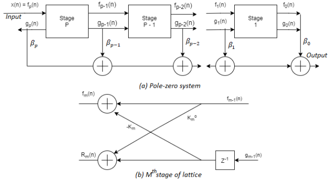
The all-pole lattice provides the basic building block for lattice type structures that implement IIR systems that has both poles and zeros. The system transfer function for IIR filter is given as
H(z) = ∑qk=0 cq(k)z-k / 1 + ∑pk=1 ap(k)z-k = Cq(z) / Ap(z)
The difference equation for the system is given by
(η) = -∑pk=1 ap(k) 𝛖(η – k) + 𝓍(η)
(η) = ∑qk=0 cq(k) 𝛖(η – k)
The output y(n) is simply linear combination of delayed outputs from all-pole systems. Since zeros result from forming a linear combination of previous outputs, we can carry over this observation to construct a pole-zero system using all-pole lattice structure as the basis of building block. The gm(n) in all-pole lattice can be expressed as a linear combination of present and past outputs. The system becomes
Hb(z) = Gm(z) / Y (z) = Bm (z)
Let the all-pole lattice filter with coefficients Km and add a ladder part by taking as the output, a weighed linear combination of {gm(n)}. The result is a pole-zero filter that has the lattice-ladder structure shown below with output as
(η) = ∑qk=0 βk gk (η)
H(z) = Y(z) / X (z) = ∑qk=0 βk Gk(z) / X(z)

Fig 1 Lattice-Ladder structure for pole-zero system
As X(z) = FP(z) and F0(z) = G0(z)
H(z) = ∑qk=0 βk Gk(z) / G0 (z) × F0(z) / Fp (z)
= 1/Ap(z) ∑qk=0 βk Bk (z)
Cq(z) = ∑qk=0 βk Bk (z)
The ladder parameter can be expressed as
Cm(z) = ∑m-1k=0 βk Bk (z) + βmBm (z)
= Cm-1(z) + βmBm (z)
When excited by a white noise sequence, this lattice-ladder filter structure generates an ARMA(p, q) process that has a power spectral density spectrum
𝗿xx () = 𝛔2 |Cq(𝒇 )|2 / |Ap(𝒇 )|2
Key takeaway
The gm(n) in all-pole lattice can be expressed as a linear combination of present and past outputs. The system becomes
Hb(z) ≣ Gm(z) / Y(z) = Bm(z)
The normal equation for the optimal filter coefficient is given by
∑M-1k=0 h(k)𝛄xx (𝒍 – k) = 𝛄dx(𝒍) 𝒍 = 0, 1, …….., M – 1
The above equation can be obtained directly by applying the orthogonality principle in linear mean square estimation. The mean square error  M in below equation is minimum if the filter coefficients {h(k)} are selected such that the error is orthogonal to each of the data point estimation.
𝓔M = E|e(𝒏)|2
= E|d(n) - ∑M-1k=0 h(k)𝒙(𝒏 – k)|
E[e(𝒏)𝒙* (𝒏 - 𝒍)] = 0 𝒍 = 0, 1, ……, M – 1
e(𝒏) = d(𝒏) - ∑M-1k=0 h(k)𝒙(𝒏 – k)
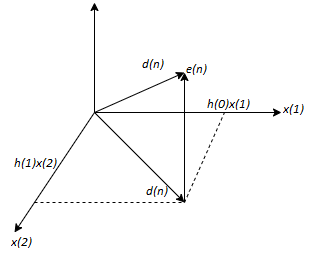
Geometrically the output of the filter is
d(n) = ∑M-1k=0 h(k)x(n-k)
The error e(n) is the vector from d(n) to  as shown in figure below.

Fig 2 Geometric representation of linear MSE
The orthogonality principle states that
𝓔M = E|e(n)|2
Is minimum when e(n) is perpendicular to the data subspace. In this case the estimated d(𝒏) can be expressed as a linear combination of the reduced set of linearly independent data points equal to the rank  The MSE is minimised by selecting the filter coefficients to satisfy the orthogonality principle the residual minimum MSE is
MMSEM = E[e(n)d*(n)]
Key takeaway
The normal equation for the optimal filter coefficient is given by
∑M-1k=0 h(k) 𝛄xx (𝒍 – k) = 𝛄dx (𝒍) 𝒍 = 0, 1, ……, M – 1
References:
1. S. K. Mitra, “Digital Signal Processing: A computer based approach”, McGraw Hill, 2011.
2. A.V. Oppenheim and R. W. Schafer, “Discrete Time Signal Processing”, Prentice Hall, 1989.
3. J. G. Proakis and D.G. Manolakis, “Digital Signal Processing: Principles, Algorithms and Applications”, Prentice Hall, 1997.
4. L. R. Rabiner and B. Gold, “Theory and Application of Digital Signal Processing”, Prentice Hall, 1992.
5. J. R. Johnson, “Introduction to Digital Signal Processing”, Prentice Hall, 1992.
6. D. J. DeFatta, J. G. Lucas andW. S. Hodgkiss, “Digital Signal Processing”, John Wiley & Sons,1988.