UNIT 2 | unit 2 discrete time systems

DSP

UNIT 2

Discrete time systems

2.1 Linear time invariant

A LTI system is one which possesses property of linear as well as time invariant system. Linear systems are one which obeys superposition theorem. There are few advantages of using LTI systems, some of which are

i) The LTI system can be easily solved mathematically for both continuous and discrete time systems.

Ii) Accurate modelling is possible in LTI system.

Iii) They are helpful for system design.

Analysis of LTI system is mainly done in two ways

a) Convolution Sum.

b) Difference Equation.

Z transform for Discrete System

Definition:

The Z transform for discrete time system x(n ) is defined as

X(z) = ------- (1) where z is a complex variable.

In polar form z can be expressed as

z = r e jw ---------------(2) where r is the radius of a circle.

For n≥ 0

X(z ) = --------- (3)which is called one-sided z-transform.

By substituting z = r e jw

X(r e jw) = (r e jw) –n ------- (4)

e- jwn ----- (5)

Equation(5) represents the Fourier transform of the signal x(n) r-n

Hence the inverse DTFT X(r ejw) must be x(n) r-n.

x(n) r-n = 1/2π r e jw ) e jwn dw

On multiplying both sides by rn we get

x(n) = 1/ 2 π r ejw) (r ejw ) n dw [ z = r ejw

Let z= r e jw and dw= dz/jz

Dz = r ejw dw

Dw = dz/jre jw

Example

Find the z-transform for the sequence

x[n] = 2 + 3 + 5 + 2

Solution:

X(z) = 2 + 3 z-1 + 5 z -2 + 2 z -3

Example

If X(z)= 4 – 5 z-2 + z-3 – 2z -4 then find x[n]

Solution:

x[n] = 4 - 5 + - 2

Example : Find the z-transform and ROC of the signal

x(n) = an u(n)

Solution:

X(z) =

= an u(n) -----(1) u(n) = 0 for n<0

1 for n≥0

= an ------- (2)

= n ------- (3)

This is a geometric series of infinite length that is

a + ar + ar2 + ………….. ∞ = a /1-r if |r| <1

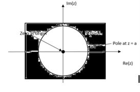
Then from equation (3) it converges when |az-1| < 1 or |z| >|a|

Therefore

X(z) = 1/ 1-az-1: ROC |z| > |a|

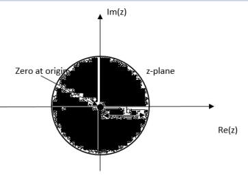
Find the z-transform of the signal x(n) =-b n u(-n-1). Find ROC

X(z) =

X(z) = bn u(-n-1) u(-n-1) =0 for n ≥0

= 1 for n ≤ -1

= bn = b-1 =

= b-1z/1- b-1z = z/ z-b = 1/ 1-bz-1 |z| < |b|

Find the z-transform of x(n) = an u(n) – bn u(-n-1)

X(z) =

= n + b-1

= z/z-a + z/z-b ROC |a| < |z| < |b|

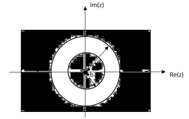
|b|< |a|

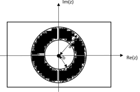
|b| >|a|

Find the z-transform of x(n) = {1,2,3,2}

Given x(0) = 1 x(1) =2 x(2) =3 x(3) = 2

X(z) =

X(z) = 1+ 2z-1 + 3 z-2 +2 z-3

Properties of Convergence

The ROC is a ring or disk in the z-plane centered at the origin.
ROC cannot contain any poles.
If x(n) is finite duration casual sequence then the ROC is the entire z-plane except at z=0.
If x(n) is finite duration anti-casual sequence then ROC is the entire z-plane except at z=∞
If x(n) is a finite duration two-sided sequence ROC is the entire z-plane except at z=0 and z=∞
If x(n) is a finite duration two-sided sequence then ROC will consist of a ring in the z-plane bounded on the interior and exterior by a pole not containing any poles.
The ROC of an LTI system contains unit circle.
ROC must be a connected region.

Find the z-transform of the signal x(n) = sin w0n u(n) and find ROC.

X(z) =

= sin = ej - e-j / 2j

= 1/2j (ejw0n – e –jwon )z-n

= 1/2j ejwon z-1) n - e-jw0z-1) n

1/2j[ 1/1-ejw0z-1 – 1/1-e-jw0z-1]

= sin w0 z-1/ 1-2cos(wo)z-1 + z-2 ROC |z| >1

LTI system

Properties of z-transform

Linearity

If X1(z) = Z{x1(n)} and X2(z) = Z{x2(n)}

Then

Z{ax1(n) + bx2(n)} = a X1(z) + b X2(z)

Proof:

Z{ax1(n) + b x2(n) }= z-n

= a z-n + b z-n

= a X1(z) + b X2(z)

Time Shifting

If X(z) = Z{x(n)} and initial conditions for x(n) are zero then

Z{x(n-m) } = z-m X(z)

Where m is a positive integer.

Proof:

Z {x(n-m)} = z-n

Let n-m = p then n= p+m

Z{x(n-m)} = z –(m+p)

z-m z-p = z-m X(z)

Multiplication by exponential sequence

If X(z ) = Z{x(n)} then

Z [ an x(n) ] = X(a-1 z)

Proof:

Z{ an x(n) } = an z-n

= (az-1)n

= X(az-1)

Convolution

We know that

Z{x(n) * h(n) } = X(z) H(z)

Proof:

Let y(n) = x(n) * h(n)

y(n)=

Taking z-transform on both sides we obtain

Y(z) = z-n

z-k z –(n-k) Replacing n-k by l

z-k z-l

= X(k) Z(k)

Time Reversal

If X(z) = Z{x(n)} then

Z{x(-n)} = X(z-1}

Proof:

Z{x(-n)} = ( z-l) -1 l=-n

= X(z-1)

Multiplication by n

If Z{x(n)} = X(z) then

Z{n x(n)} = -z d/dz X(z)

X(z) =

Z{n x(n)} =

= z -1

= z

= -z }

= -z d/dz {

= -z d/dz X(z)

Problems:

Find the z-transform of the sequence

x(n) = a n-1 u(n-1)

We know that x(n) = an u(n) is

X(z) = 1/1/az-1

By using time shifting property we have Z{ x(n-k)} = z-k X(z)

Therefore

Z{an-1 u(n-1)} = z-1/ 1-az-1 = 1/z-a. ROC |z| > |a|

Find the z-transform of the sequence

x(n) = an cos nπ/2

Z{ cos w0n} = 1- (cos w0) z-1/ 1 –(2 cos w0) z-1 + z-2

Since w0=π/2

Z{ cos π/2 n u(n)} = 1/1 + z-2

Using exponential sequence property

Z{ an x(n) } = X(a-1 z)

Z{ an cos nπ/2} = 1/1+(a-1z)-2 = 1/ 1 + a2/z2 = z2/ a2 + z2

Find the z transform of the sequence x(n) = n u(n)

The z-transform of unit step sequence is given by

Z{u(n)} = z/z-1

Z{ n u(n)} = -z d/dz (z/z-1)

= z/(z-1)2

If x(n) = x1(n) * x2(n) where x1(n) = (1/3)n u(n) and x2(n) = (1/5)n u(n). Find X(z) by using convolution property.

X1(z) = 1/ 1- (1/3)z-1 X2(z) = 1/1- (1/5) z-1

X(z) = 1/1-(1/3)z-1 . 1/1-(1/5) z-1

Using z-transform find the convolution of two sequences.

x1(n) = {1,2,-1,0,3} x2(n) = { 1,2,-1}

Z{ x1(n) * x2(n)} = X1(z) . X2(z)

X1(z) = 1 + 2z-1 – z-2 + 3 z-4

X2(z) = 1 + 2z-1 – z-2

(1 + 2z-1 – z-2 + 3 z-4 ) (1 + 2z-1 – z-2 )

= 1 + 4z-1 + 2z-2 – 4 z- 3 + 4 z-4 + 6 z- 5 – 3 z-6

Determine the z-transform of the signal

x(n ) = rn (sin w0n ) u(n)

Z{(sin w0n ) u(n)} = sin w0 z-1/ 1 -2 (cos w0) z-1 + z-2

Z{ an x(n)} = X(a-1 z)

Therefore

Z{ rn sin(w0n) u(n) } = (sin w0) (r-1 z)-1/ 1- 2 (cos w0)(r-1z)-1 + (r-1z)-2

= r(sinw0) z-1/ 1-2r(cos w0) z-1 + r2 z-2

Determine the signal x(n) whose z-transform is given by

X(z) = log(1- az-1)

X(z)= log(1-az-1)

Differentiating both sides we get

d/dz X(z) = 1/1-az-1 (a z-2) = az-2/1- az-1

-z d/dz { X(z)} = -az-1/1-az-1

= -az-1[ 1/1-az-1]

= -a Z[ a n-1 u(n-1)] -------- (1)

From differentiation property

Z{ n x(n)} = -z d/dz [ X(z)] ------- (2)

Comparing (1) and (2) we get

n x(n) = -a [ a n-1 u(n-1)]

Or x(n) = -a [a n-1 u(n-1)]/n

Determine the z-transform of the signal

x(n) =1/2 (n2 + n) (1/3) n-1 u(n-1)

=½ n2 (1/3) n-1 u(n-1) +1/2 n (1/3) n-1 u(n-1)

We know that

Z[(1/3) n u(n)] = z/ z-1/3

Using time-shifting property

Z{(1/3) n-1 u(n-1)] = 1/ z- 1/3

Z [ n (1/3) n-1 u(n-1)] = -z d/dz [1/z-(1/3)]

=-z d/dz( 1/z-1/3)= -z [-1/(z-1/3) 2]= z/ (z-1/3)2

Z [ n2 (1/3) u(n-1)] = -z d/dz [ z/(z-1/3)2]

= z(z+1/3)/(z-1/3)2

= -z [ (z-1/3)2 -2z(z-1/3)/(z-1/3)4

= z(z+1/3)/(z-1/3)3

X(z) = ½[z(z+1/3)/(z-1/3)3 + z/ (z-1/3)2]

= z2/(z-1/3)3

Inverse Z-transform

There are three methods that are often used to find inverse z-transform.

Long Division Method
Partial fraction method
Convolution Method

Long Division Method

If X(z) is the ratio of two polynomials then

X(z) = N(z)/D(z ) = b0 + b1 z-1 + b2 z-2 +……….. +bM z-M

1+ a1z-1 + a2 z-2 + …………. + aN z-N

Using long division method Find the inverse z-transform of the sequence of

X(z) = z+1

z2 +3z + 2

z-1 + 4z-2 + 10 z-3 +22 z-4

z2 -3z +2 z+1

z- 3 + 2z-1

4 – 2z-1

4 – 12 z-1 + 8 z-2

10z-1 – 8z-2

10 z-1 – 30z-2 +20 z-3

22 z-2 – 20 z-3

22 z-2 -66 z-3 +44 z-4

46 z-3 – 44 z-4

X(z) = z-1 + 4 z-2 + 10 z-3 + 22z-4

x(n) = { 0,1,4,10,22………}

Partial fraction Method

Find the partial fraction method of

X(z) = ¼ z-1

(1 – ½ z-1)(1-1/4 z-1)

X(z) = A + B

Z (1-1/2z-1) (1 – ¼ z-1)

By solving A= 1 and B=-1

Therefore,

X(z) = z - z

z-1/2 z-1/4

x(n) = (1/2) n u(n) – (1/4) n u(n)

Find the partial fraction of

X(z) = 1

1+ z-1 + z-2

X(z) = z

z2 + z + 1

= z

(z + 0.5 +j 0.866)(z+0.5 – j0.866)

X(z) = c + c*

z z-(-0.5 +j0.866) z – (- 0. 5 – j 0.866)

X(z) = 0.5+j0.288 + 0.5 – j 0.288

z z-(-0.5 +j0.866) z – (- 0. 5 – j 0.866)

X(z) = 0.5+j0.288 z + 0.5 – j 0.288 z

z-(-0.5 +j0.866) z – (- 0. 5 – j 0.866)

By taking inverse z-transform both sides we get

= (0.5+j0.288)( (-0.5 +j0.866) n u(n) +(0.5+j0.288)( (-0.5 -j0.866) n u(n)

2.2 Response of LTI system convolution sum

Considering an LTI system with input as impulse signal. As we know that impulse response of any system gives complete describes the behavior of any LTI system. Basically, we decompose the input signal first. The apply input as impulse and obtain the corresponding output. Obtained output is then graphically analyzed.

Let input signal be x[n]

x[n] =

The output obtained when we apply input as unit sample sequence for n=k

y[n,k] = h[n,k] = H[[n-k]]

Where n= time index

k = location of input impulse parameter

The x[n] because of input weighted sum of output will be

y[n] = H[x[n]]

= H [ ]

But y[n,k] = h[n,k] = H[[n-k]]

Hence, the output will now be

y[n] = [ ]

= ] (Due to superposition theorem)

Now, by time invariance property we can write

h[n]= H [

For delayed sequence we have

h[n-k] =H []

Hence, the output equation can now be written as

y[n] = [ ]

The above equation is called as convolution sum.

y[n]= x[n] * h[n]

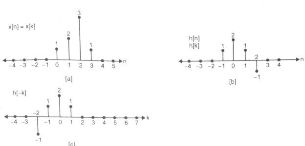
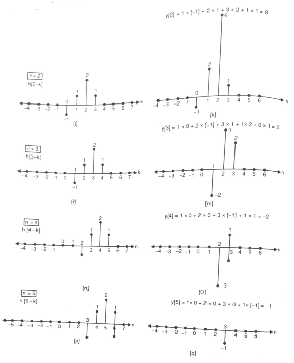
Que) For sequence h[n]={ 1, 2 , 1, -1} determine the response of system with input signal x[n] = {1, 2 ,3 ,1}

Sol:

a) Finding x[k] and h[k] i.e n=k.

b) Folding h[k] we get h[-k].

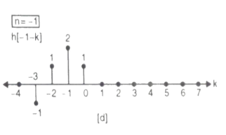
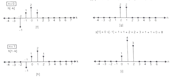
c) Then shifting the above signal[-k] we get h[1-k]

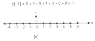
d) Multiplying above signal h[1-k] with x[n].

e) Again, incrementing h[1-k] by 1 we get h[2-k] multiplying with x[n].

f) Continuing this process till we get 0 for output y. In this case for n=5.

The graphical representation is shown below.

Convolution by tabulation method

In this method we form a table type structure and find the convolution of x[n] and h[n]. We will understand this by solving an example.

Que) For h[n] = {1, 2, 1, -1}, x[n] = {1, 2, 3, 1}. Find x[n]*h[n]?

Sol:

1 2 3 1

1 1 2 3 1

2 2 4 6 2

1 1 2 3 1

-1 -1 -2 -3 -4

y[-1] = 1

y[0]= 2+2 = 4

y[1] = 1+4+3 = 8

y[2]= -1+2+6+1 = 8

y[3]= -2+3+2 = 3

y[4]= -3+1 = -2

y[5]= -1

y[n]= {1, 4, 8, 8, -2, -1}

The above sequence is the required convolution of x[n] and h[n].

2.3 Description of discrete time system by difference equation and complete solution of difference equation

The general nth order difference equation is given as

a0y[n]+ay[n-1]+….+aN-1y[n-N+1]+any[n-N]=b0x[n]+b1x[n-1]+….+bMx[n-M]

The difference equation can be written as

The output equation can be given as

y[n] = { - }

The above difference equation can be solved by finding homogeneous and particular solution or by z transform method. Z transform is discussed in above section.

Homogeneous Solution:

Let x[n]=0

The solution to above equation will be of the form y[n] = rn

Then solution will be of the form

y[n] = p1 + p2+ p3+……+ pn (For distinct roots)

y[n]= p1n + p2+ p3+……+pm+1+…….+ pnrN (For multiple roots)

Que) Find the homogenous solution for the difference equation y[n]-y[n-1]+y[n-2]=1+3-n. Given y[-2] = 0 and y[-1]=2

Sol: For homogeneous solution

Y[n] = rn

rn-rn-1+rn-2 = 0

rn-2(r2-r+) = 0

Solving above equation we get

r= and r=1

Roots are distinct so the solution will be of the form

y[n] = p1 + p2

y[n] = p12-n +

Particular Solution:

The complete solution of any difference equation is the sum of homogeneous solution and the particular solution.

Que) For the difference equation find the particular solution x[n] = 3n

y[n] = x[n]+y[n-1]- y[n-2]?

Sol: As x[n] = 3n

From table the particular solution will be y[n] = k3n

y[n] = x[n]+y[n-1]- y[n-2]

k3nu(n) = 3nu(n)+ k 3n-1u(n-1)-k3n-2u(n-2)

Finding k for n≥2

K 32 = 32+ k 32-1- k 32-2

9k-k+k = 9

k= 27/20

y[n]= 3n

2.4 Implementation of discrete time systems

The basic realization techniques used for filters are direct form, cascade form and parallel form. In this section we will study all in detail. This section overviews ability to implement finite impulse response (FIR) and infinite impulse response (IIR) filters using different structures in terms of block diagram and signal flow graph.

For an LTI system the transfer function is given as

H(z)= (1)

The difference equation can be written as

(2)

x(n)= system input

y(n)=system output

When a0≠ (3)

The above equation implementation requires some basic blocks shown below

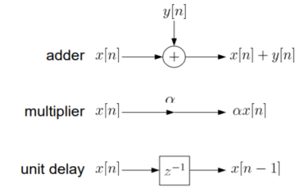
Fig: Block diagram representation

The above blocks can be easily understood with the help of one example. For the standard LTI system with difference equation

Y[n]=-a1y[n-1]-a2y[n-2]+b0x[n]. Draw the block diagram for the given equation.

Sol: We already know that x[n] and y[n] are the input and output to the system respectively.

If we need the term y[n-1] we need a delay block after y[n], and one more delay block after y[n-1] to get y[n-2].
For getting term -a1y[n-1] we need multiplier of -a1and same for -a2.
To get complete term -a1y[n-1]-a2y[n-2]+b0x[n] we need adders so that the we get the final equation.
The final figure using 2 adders, 3 multipliers and 2 delay block is shown below.

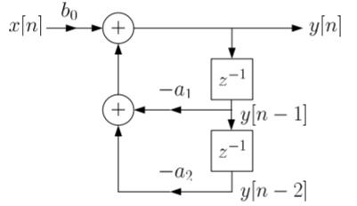
Fig: Block diagram representation

FIR FILTER:

The standard equation for representing the FIR filter is shown below

H(z)= (4)

From equation (1) and (4) we can conclude that FIR filters do not contain any pole. The difference equation will be

Y[n]= (5)

a) Direct Form:

The direct form is directly derived from the difference equation. It can be represented as

y[n]= (6)

Where h(k) is the system impulse response.

Expanding the above equation, we get

Y[n]==h[0]x[n]+h[1]x[n-1]+……h[M]x[n-M] (7)

The block diagram representation for above direct form is shown below.

Fig: Direct form realization of Fir filter

b) Cascade Form:

As we already know H(z)=

The above equation can be represented as a product of second order polynomial as

H(z)== (8)

Mc=|(M+1)/2|

The above equation can be further simplified with intermediate output of system 1 w1(n) fed to the input of second cascade structure and so on.

The difference equation is given as

w1(n)= + (9)

w2(n)= + (10)

Fig: Cascade form FIR filter

IIR FILTER:

The transfer function of IIR filter is given as

H(z)= (11)

From above equation we can conclude that an IIR filter contains at least one pole.

a) Direct Form:

The direct form is realised directly from its difference equation

v[n]= (12)

y[n]=- +v[n] (13)

Another way to obtain direct form is by decomposing H(z) into two transfer functions

H(z)=H1(Z). H2(z)

H1(Z)= (14)

H2(z)= (15)

V(z)=X(z). H1(Z)=X(z) (16)

Y(z)=V(z). H2(z)=V(z) (17)

The final realisation block diagram representation of direct form for IIR filter is shown below

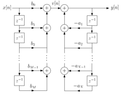
Fig: Direct Form realization of IIR Filter

b) Cascade form:

To find the transfer function for cascade for we need to factorize the numerator and denominator polynomials in terms of second order polynomial.

H(z)== (18)

Nc=|(N+1)/2|

Let us consider M=N=4. Then the cascade realisation for IIR filter is shown below.

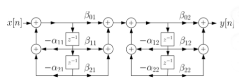
Fig: Cascade Form realisation of IIR Filter

Que) For the following LTI system H(z)= . Realise the cascade form IIR filter.

Sol: H(z)=

The above function can be simplified as

H(z)=

Hence, using the above structure and placing the values of …. And similarly,

c) Parallel form:

The parallel form is given as H(z)=+ (19)

Nc=(N=2)/2

Que) Draw block diagram for the function using parallel form H(z)=

Sol: H(z)=

Writing above transfer function in standard form for parallel realisation we get

H(z)=-20+

The structure is shown below

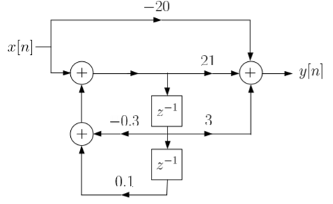
2.5 Correlation of discrete time signals

Correlation means to correlate two signals or processes. In correlation we just reverse one of the sequences. There are two types in which we can correlate signals as mentioned below.

Mathematically correlation can be defined as

rxy(l) =