Unit 3
Frequency Domain Analysis
It gives the frequency response of the system. If the transfer function is given, than from the plot number of poles and zeros can be calculated.
Polar plot of some standard functions :-
# TYPE ‘O’
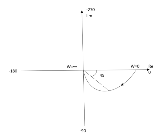
Ex : 1T(S) = 1/S + 1
(1). For polar plot substitute S=jw.
TF = 1/1 + jw
(2). Magnitude M = 1 + 0j / 1 + jw = 1/√1 + w2
(3). Phase φ = tan-1(0)/ tan-1w = - tan-1w
W M φ
0 1 00
1 0.707 -450
∞ 0 -900
The plot is shown in fig. 3(a)
Ex.2>. T(S) = 1/(S+1)(S+2)
(1). S = jw
TF = 1/(1+jw)(2+jw)
(2). M = 1/(1+jw)(2+jw) = 1/-w2 + 3jw + 2
M = 1/√1 + w2√4 + w2
(3). Φ = - tan-1 w - tan-1(w/2)
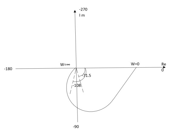
W M Φ
0 0.5 00
1 0.316 -71.560
2 0.158 -108.430
∞ 0 -1800
The plot is shown in fig3(b)
Intersection of polar plot with imaginary axis will be when realpart of Transfer function = 0
M = 1/(jw + 1)(jw + 2)
= 1/-w2 + j3w + 2
Real part
Re(M) = 1/(2-w2)+j3w x (2-w2)-3jw/(2-w2)-3jw
Re(M) = (2-w2)/(2-w2+9w2) - 3jw/(2-w2) +9w2
Equating Real part = 0
(2-w2)/(2-w2)+ 9w2 = 0
W = +-√2
For w=√2 real part on the polar plot becomes zero.
So, polar plot intersects imaginary axis at w=√2 at φ = -900
Ex.3 T(S) = 1/(S+1)(S+2)(S+3)
(1). Substitute S =jw
(2). M = 1/√1+w2 √4+w2 √9+w2
(3). Φ = -tan-1w – tan-1 w/2 – tan-1w/3
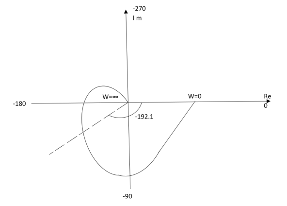
W M φ
0 0.16 0
1 0.1 -900
2 0.04 -142.10
∞ 0 -270
(4). Intersection of Polar plot with Real axis
M = 1/(S+1)(S+2)(S+3)
= 1/S3+6S2+11S+6
=1/(jw)2+6(jw)2+11jw+6
= 1/(6-6w2)+j(11w-w3)
Re(M) = 0 [Intersection with imaginary axis ]
M = 6-6w2/(6-6w2)2+(11w-w2)2 - j(11w-w3)/(6-6w2)2+(11w-w2)2
Re(M) = 0
6-6w2 = 0
w=1
Im(M) = 0[Intersection with Real axis]
11w = w3
The plot is shown in fig 3(c)
TYPE ‘1’
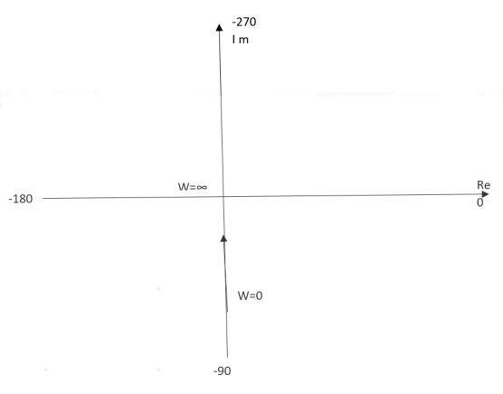
Ex.1 T(S) = 1/S
(1). S = jw
(2). M = 1/W
(3). Φ = -tan-1(W/O) = -900
W M φ
0 ∞ -900
1 1 -900
2 0.5 -900
∞ 0 -900
The plot is shown in fig.4(a)
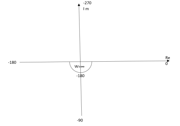
Ex.2 T(S) = 1/S2
(1). S = jw
(2). M = 1/w2
(3). Φ = -tan-1(W/O)-tan-1(W/O) = -1800
W M Φ
0 ∞ -1800
1 1 -1800
2 0.25 -1800
∞ 0 -1800
The plot is shown in fig.4(b)
- For Polar Plot starting point depends upon type of system
- The terminating phase depends on order of the system.
TYPE 1 ORDER 2
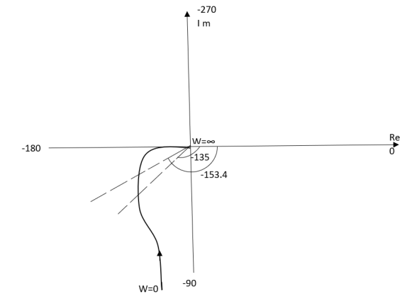
Ex.1 T(S) = 1/S(S+1)
(1). M = 1/W√1+w2
(2). Φ = -900 - tan -1(W/T)
W M φ
0 ∞ -900
1 0.707 -1350
2 0.45 -153.40
∞ 0 -1800
The plot is shown in fig.5(a)
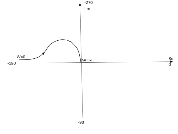
Ex.2TYPE 2 ORDER 3
T(s) = 1/S2(S+1)
(1). M = 1/w2√1+jw
(2). Φ = -1800 – tan-1W/T
The plot is shown in fig.5(b)
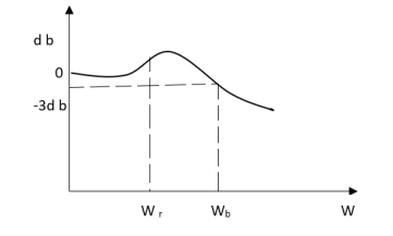
(1). Resonant Frequency Wr
(2). Resonant Peak (Mr)
(3). Bandwith (WO)
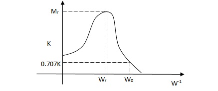
(1). Resonant Freq
It is frequency at which CL system magnitude is maximum.
(2). Resonant Peak
Max magnitude of CL system is called Mr.
(3). BW
It is range of freq whose CL sys mag >/ 0.707 times the 0 freq. Mag.
CLTF = w2n/S2 + 2 ξwnS + w2n
CLTF = w2n/-w2 + j2 ξwnw + w2n
= 1/-(w/wn)2 + j2 ξw/wn + 1
= 1/1 - µ2 + 2 ξµj
|µ| = 1/√(1-µ)2 + (2 ξµ)2
d µ/d µ = 0
µ = √1 - 2 ξ2
w/wn = √1 - 2 ξ2
wr = wn√1 - 2 ξ2
|Mr| = 1/√(1 – (w/wn)2)2 + (2 ξw/wn)2
|Mr| = 1/2 ξ√(1 –ξ2
BW = wr[1 – 2G2S + √4ξ4 + 4ξ2 + 2]1/2
In polar plot any point gives the magnitude phase of the transfer function in bode we split magnitude and  plot.
plot.
Advantages
- By looking at bode plot we can write the transfer function of system
Q. G(S) = 
1. Substitute S = j
G(j ) =
) = 
M = 
 = tan-1
 = -900
Magnitude varies with ‘w’ but phase is constant.
MdB = +20 log10

Decade frequency :-
W present = 10  past
past
Then  present is called decade frequency of
  past
past
 2 = 10
  1
1
 2 is decade frequency of
  1
1
 MdB
MdB
0.01 40
0.1 20
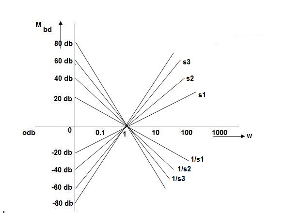
1 0 (shows pole at origin)
0 -20
10 -40
100 -60
Slope = (20db/decade)
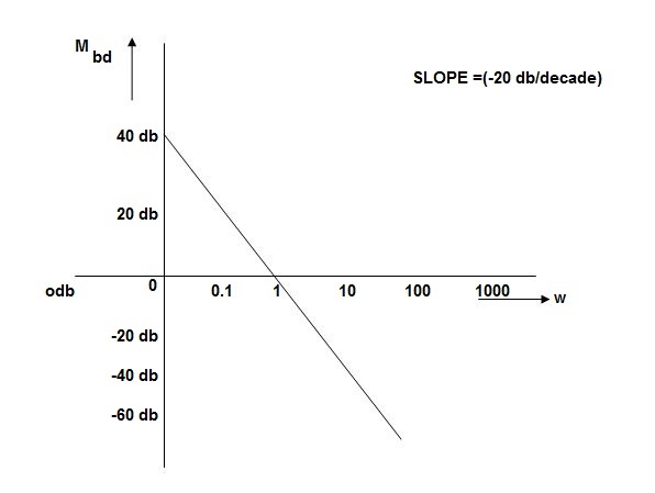
MAGNITUDE PLOT
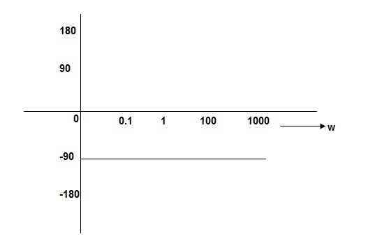
PHASE PLOT
Q.G(S) = 
G(j ) =
) = 
M =  ;
;  = -1800 (-20tan-1
 )
)
MdB = +20 log  -2
-2
MdB = -40 log10
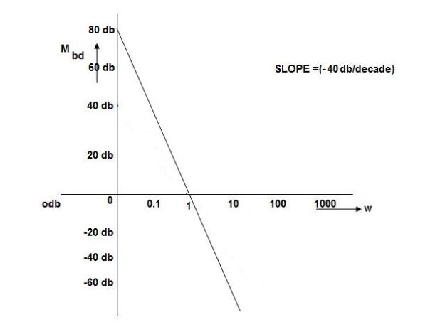
 MdB
MdB
0.01 80
0.1 40
1 0 (pole at origin)
10 -40
100 -80
Slope = 40dbdecade
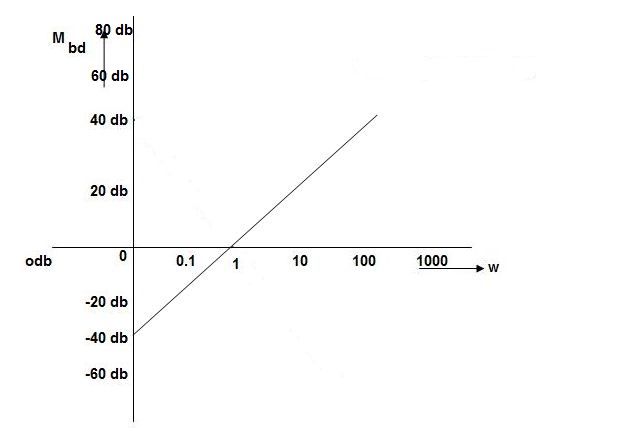
Q. G(S) = S
M= W
 = 900
= 900
MdB = 20 log10
 MdB
MdB
0.01 -40
0.1 -20
1 0
10 20
100 90
1000 60
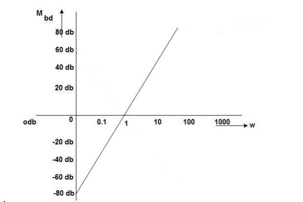
Q. G(S) = S2
M=  2 MdB = 20 log10
 2
2
 = 1800 = 40 log10
W MdB
0.01 -80
0.1 -40
1 0
10 40
100 80
Q. (S) = 
G(j ) =
) = 
M = 
MdB = 20 log10 K-20 log10
 = tan-1(
 ) –tan-1(
 )
)
 = 0-900 = -900
K=1 K=10
 MDb MdB
=-20 log10 =20 -20 log10
0.01 40 60
0.1 20 40
1 0 20
10 -20 0
100 -40 -20
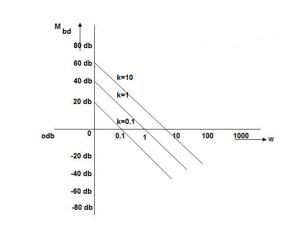 As we vary K
  then plot shift by 20 log10K
i.e adding a d.c. To a.c. Quantity
Approximation of Bode Plot:
IF poles andzeros are not located at origin
G(S) = 
TF = 
M = 
MdB = -20 log10 (
 = -tan-1
Approximation:  T >> 1. So, we can neglect 1.
MdB = -20 log10
MdB = -20 log10 T . ;
T . ;  = -tan-1(
 T)
T)
Approximation:  T << 1. So, we can neglecting
 T.
T.
MdB= 0dB,  = 00
= 00
At a point both meet so equal i.e a time will come hence both approx become equal
-20 log10 T= 0
T= 0
 T= 1
T= 1
 corner frequency
At this frequency both the cases are equal
MdB = -20 log10
Now for 
MdB = -20 log10
= -20 log10
= -10 log102
MdB = 10
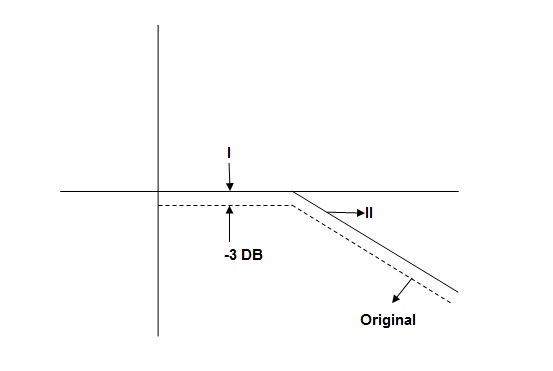
When we increase the value of  in app 2 and decrease the
  of app 1 so a RT comes when both cases are equal and hence for that value of
  where both app are equal gives max. Error we found above and is equal to 3dB
At corner frequency we have max error of -3dB
Q. G(S) = 
TF = 
M = 
MdB = -20 log10 ( at T=2
 MdB
MdB
1 -20 log10
10 -20 log10
100 -20 log10
 MdB
MdB  =
= =
= 
0.1 -20 log10 = 1.73
  10-3
10-3
0.1 -20 log10 = -0.1703
0.5 -20 log10 = -3dB
1 -20 log10 = -6.98
10 -20 log10 = -26.03
100 -20 log10 = -46.02
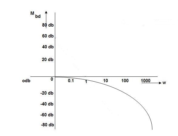
Without approximation
For second order system
TF = 
TF = 
= 
= 
= 
M= 
MdB= 
Case 1  <<
<<
 << 1
<< 1
MdB= 20 log10 = 0 dB
Case 2  >>
>>
 >> 1
>> 1
MdB= -20 log10
= -20 log10
= -20 log10
 < 1
< 1  is very large so neglecting other two terms
MdB= -20 log10
= -40 log10
Case 3 . When case 1 is equal to case 2
-40 log10 = 0
= 0
 = 1
= 1

The natural frequency is our corner frequency
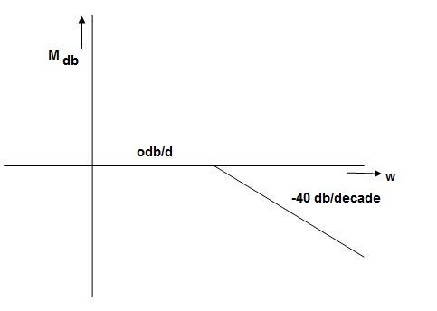
Max error at  i.eat corner frequency
MdB= -20 log10
For 
MdB= -20 log10 
 error for
Completely the error depends upon the value of  (error at corner frequency)
The maximum error will be
MdB= -20 log10 
M = -20 log10 
 = 0
= 0

 is resonant frequency and at this frequency we are getting the maximum error so the magnitude will be
M = - +
+ 
= 
Mr =
MdB= -20 log10
MdB= -20 log10 
 = tan-1

Mr = 
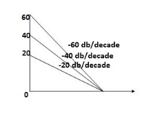
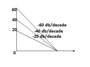
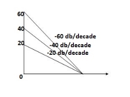
Type of system | Initial slope | Intersection |
0 | 0 dB/decade | Parallel to 0 axis |
1 | -20 dB/decade | =K1 |
2 | -40 dB/decade | =K1/2 |
3 | -60 dB/decade | =K1/3 |
. | . | 1 |
. | . | 1 |
. | . | 1 |
N | -20N dB/decade | =K1/N |
Sketching of Bode Plot:
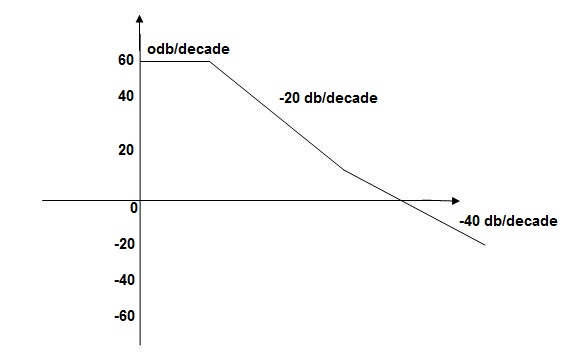
Q.1 sketch the bode plot for transfer function
G(S) = 
- Replace S = j

G(j =
= 
This is type 0 system . So initial slope is 0 dB decade. The starting point is given as
20 log10 K = 20 log10 1000
= 60 dB
Corner frequency  1 =
1 =  = 10 rad/sec
 2 =
2 =  = 1000 rad/sec
Slope after  1 will be -20 dB/decadetill second corner frequency i.e
 2 after
  2 the slope will be -40 dB/decade (-20+(-20)) as there are poles
2. For phase plot
 = tan-1 0.1
 - tan-1 0.001
For phase plot


100 -900
200 -9.450
300 -104.80
400 -110.360
500 -115.420
600 -120.00
700 -124.170
800 -127.940
900 -131.350
1000 -134.420
 The plot is shown in figure 1
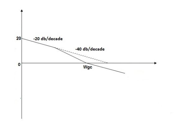
Q.2 for the given transfer function determine
G(S) = 
Gain cross over frequency phase cross over frequency phase mergence and gain margin
Initial slope = 1
N = 1 , (K)1/N = 2
K = 2
Corner frequency
 1 =
1 =  = 2 (slope -20 dB/decade
 2 =
2 =  = 20 (slope -40 dB/decade

2. phase
 = tan-1
 - tan-1 0.5
  - tan-1 0.05
 = 900- tan-1 0.5
  - tan-1 0.05


1 -119.430
5 -172.230
10 -195.250
15 -209.270
20 -219.30
25 -226.760
30 -232.490
35 -236.980
40 -240.570
45 -243.490
50 -245.910
Finding  gc (gain cross over frequency
M = 
4 =  2 (
2 ( (
(
 6 (6.25
 104) + 0.252
 4 +
4 + 2 = 4
2 = 4
Let  2 = x
2 = x
X3 (6.25 104) + 0.252
 2 + x = 4
X1 = 2.46
X2 = -399.9
X3 = -6.50
For x1 = 2.46
 gc = 3.99 rad/sec(from plot )
For phase margin
PM = 1800 -
 = 900 – tan-1 (0.5×
 gc) – tan-1 (0.05 ×
  gc)
gc)
= -164.50
PM = 1800 - 164.50
= 15.50
For phase cross over frequency ( pc)
pc)
 = 900 – tan-1 (0.5
  ) – tan-1 (0.05
  )
)
-1800 = -900 – tan-1 (0.5  pc) – tan-1 (0.05
  pc)
pc)
-900 – tan-1 (0.5  pc) – tan-1 (0.05
  pc)
pc)
Taking than on both sides
Tan 900 = tan-1
Let tan-1 0.5  pc = A, tan-1 0.05
  pc = B
 = 00
= 00
 = 0
= 0
 1 =0.5
  pc 0.05
 pc
pc
 pc = 6.32 rad/sec
The plot is shown in figure 2
Q3. For the given transfer function
G(S) = 
Plot the rode plot find PM and GM
T1 = 0.5  1 =
1 =  = 2 rad/sec
Zero so, slope (20 dB/decade)
T2 = 0.2  2 =
2 =  = 5 rad/sec
Pole , so slope (-20 dB/decade)
T3 = 0.1 = T4 = 0.1
 3 =
3 =  4 = 10 (2 pole ) (-40 db/decade)
- Initial slope 0 dB/decade till
 1 = 2 rad/sec
 - From
 1 to
1 to 2 (i.e. 2 rad /sec to 5 rad/sec) slope will be 20 dB/decade
 - From
 2 to
2 to  3 the slope will be 0 dB/decade (20 + (-20))
 - From
 3 ,
3 , 4 the slope will be -40 dB/decade (0-20-20)
Phase plot
 = tan-1 0.5
 - tan-1 0.2
 - tan-1 0.1
 - tan-1 0.1


500 -177.30
1000 -178.60
1500 -179.10
2000 -179.40
2500 -179.50
3000 -179.530
3500 -179.60
GM = 00
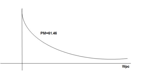
PM = 61.460
The plot is shown in figure 3
Q 4.For the given transfer function plot the bode plot (magnitude plot)
G(S) = 
Given transfer function
G(S) = 
Converting above transfer function to standard from
G(S) = 
= 
- As type 1 system , so initial slope will be -20 dB/decade
- Final slope will be -60 dB/decade as order of system decides the final slope
- Corner frequency
T1 =  ,
,  11= 5 (zero)
T2 = 1 , 2 = 1 (pole)
4. Initial slope will cut zero dB axis at
(K)1/N = 10
i.e = 10
= 10
5. finding  n and
n and 
T(S) = 
T(S)= 
Comparing with standard second order system equation
S2+2 ns +
ns + n2
n2
 n = 11 rad/sec
 n = 5
n = 5
 11 = 5
 =
=  = 0.27
5. Maximum error
M = -20 log 2
= +6.5 dB
6. As K = 10, so whole plot will shift by 20 log 10 10 = 20 dB
 The plot is shown in figure 4
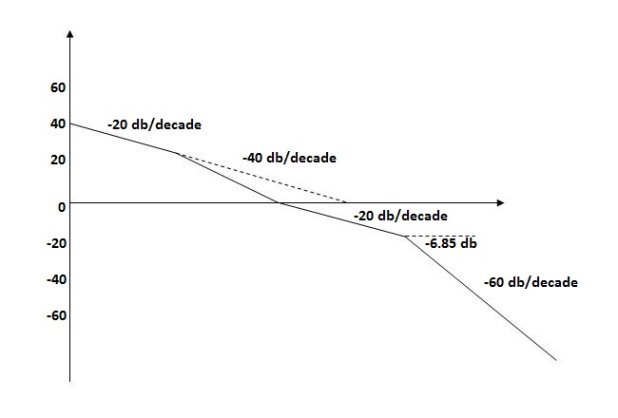
Q5. For the given plot determine the transfer function
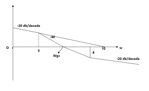
From figure 5 we can conclude that
- Initial slope = -20 dB/decade so type -1
- Initial slope alls 0 dB axis at
 = 10 so
K1/NN = 1
(K)1/N = 10.
3. corner frequency
 1 =
1 =  = 0.2 rad/sec
 2 =
2 =  = 0.125 rad/sec
3. At  = 5 the slope becomes -40 dB/decade, so there is a pole at
  = 5 as
Slope changes from -20 dB/decade to -40 dB/decade
4. At  = 8 the slope changes from -40 dB/decade to -20 dB/decade hence
5. is a zero at  = 8 (-40+(+20)=20)
6. Hence transfer function is
T(S) = 
Correlation with time domain performance
The transfer function of second order system is given as
C(s)/ R(s) = wn2/s2+2 wns+wn2 (1)
 =damping factor
wn=undamped natural frequency
For frequency response let s=jw

Let u= the above equation becomes
T(j )=
)=
|T(j )|=M=1/
 (2)
(2)
 =φ=-tan-1[
 /
/ ] (3)
] (3)
For sinusoidal input the output response for the system is given by
c(t)= sin[
sin[ t-tan-1[
 /
/ ] (4)
] (4)
The frequency where M has the peak value is known as Resonant Frequency  . This frequency is given as from equation (2)
 (5)
(5)
From equation (2) the maximum value of magnitude is known as Resonant Peak
Mr= (6)
(6)
The phase angle at resonant frequency is given as
φr=-tan-1[ (7)
(7)
As we already know for step response of second order system the value of damped frequency and peak overshoot are given as
 (8)
(8)
Mp= (9)
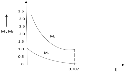
(9)
The comparison of Mr and Mp is shown if figure below. The two performance indices are correlated as both are function of damping factor. When subjected t step input the system with given value of Mr of its frequency response will exhibit a corresponding value of Mp.
Similarly, the correlation of  and
and  is also shown below. For the given input step response [equation (5) and (6)]

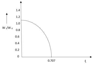
Mp= Peak overshoot of step response
Mr = Resonant peak of frequency response
 =Resonant frequency of frequency response
 =Damping frequency of oscillations of step response
The transfer function of the plant should be known. It becomes difficult to infer all the performance values. When the input is sinusoidal it becomes difficult to get steady state response.
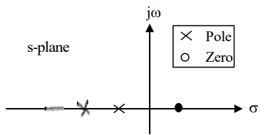
The transfer function of Minimum phase system has neither poles or zeros in the right half of s-plane. In these systems the magnitude and phase characteristics can be uniquely related.
G(s) = 
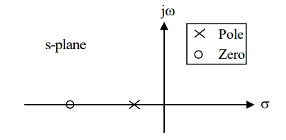
The transfer function of Non-Minimum phase transfer function has at least one pole or zero on the right half of s-plane. The non-minimum phase systems are very slow in response.
G(s) = 
