Unit 5
Control System Analysis using State Variable Methods
The above figure shows the state model of a system with two inputs u1(t) and u2(t), and having outputs y1(t) and y2(t). We know that the output equation is given as
Y(t)=Cx(t)+Du(t) (1)
 (2)
(2)
Taking L.T of equation (1)
Y(s)=CX(s)+DU(s) (3)
Taking L.T of equation (2)
SX(s)=AX(s)+BU(s) (4)
X(s)=[SI-A]-1BU(s) (5)
Y(s)=CX(s)+DU(s)
Y(s)=C{[SI-A]-1BU(s)} + DU(s)
 = C{[SI-A]-1B} + D (6)
[SI-A]-1=
The denominator of equation (6) is the characteristic equation
[SI-A]=0
Q1) For the given data below compute the transfer function of the system
A= B=
B= C=[1 0] and D=[0]
Sol: The state equation will be
 =
= +
+
 =x1
=x1
 =-6x1-5x2
 = C{[SI-A]-1B} + D
=C{ -
- }-1B+D
=C B+D
B+D
=[1 0]  + 0
+ 0
= +0
+0
 =
=
Q.1) A= . Calculate characteristic equation and stability?
Sol: The characteristic equation is given as [SI-A]=0
S -
-  =0
=0
 -
- = 0
= 0
 =0
=0
S(S+3)-(-1)*2=0
Hence, the characteristic equation is
S2+3S+2=0
(S+1)(S+2)=0
S=-1,-2
Both roots on left-half of s-plane, real and different, system absolutely stable.
Q.2)A=  Find the characteristic equation and comment on stability?
Sol: The characteristic equation is given by [SI-A]=0
 -
- =0
=0
 =0
=0
S(S+2)+2=0
S2+2S+2=0
S=-1±j
Roots on left-half of s-plane, complex conjugate, system absolutely stable.
This can be implemented by three ways as listed below:
a) By Block diagram method (Jordan’s Canonical form)
b) By Signal flow graph
c) By differential equation
By Block diagram method (Jordan’s Canonical form)
Q1) The closed loop transfer function is given as T(s)= . Calculate the state model?
Sol: The transfer function can be simplified using partial fraction method as
 =
=
S+2=As+10A+Bs+5B
Equating coefficients of s from both sides
A+B=1
Equating coefficients of s0 from both sides
10A+5B=2
Solving above equations we get
A=-3/5
B=8/5
The transfer function will be
T(s)=
=- +
+
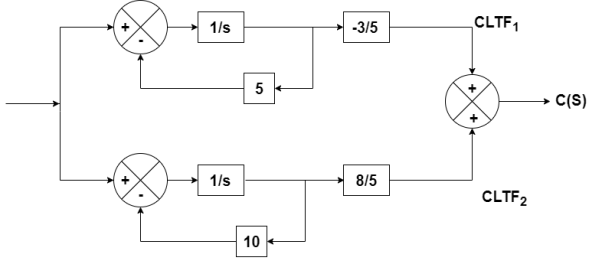
Number of poles= Number of energy storing elements
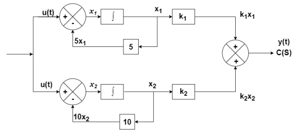
The output equation is given as
y(t)=k1x1(t)+k2x2(t)
y(t)= [k1 k2] + [0] [u(t)]
y(t)= [-3/5 8/5] + [0] [u(t)]
C=[-3/5 8/5]
D=0
From the above block diagram
 =u(t)-5x1
 =-5x1+u(t)
 =-10x2+u
Therefore, the state equation is given as
 =
= +
+
A=
B=
Q2) The closed loop transfer function is given as T(s)= . Calculate the state model?
Sol: The transfer function can be simplified using partial fraction method as
 =
= +
+ 
s+7=A[s2+7s+12] +B[s2+6s+8] +C[s2+5s+6]
Equating coefficients of s2 from both sides
A+B+C=0
Equating coefficients of s from both sides
7A+6B+5C=1
Equating coefficients of s0 from both sides
12A+8B+6C=7
Solving above equations and finding values of A, B and C
A=5/2
B=-4
C=3/2
The transfer function will be
T(s)= +
+ 
= +
+ 
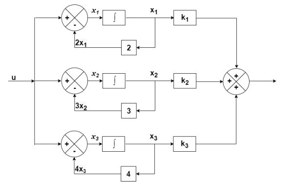
The output equation will be
y=k1x1+k2x2+k3x3
y=[k1 k2 k3] [5/2 -4 3/2]
C=[5/2 -4 3/2]
D=[0]
The state equation is given as
 =u(t)-2x1
 =-2x1+u(t)
 =-3x2+u
 = -4x3+u
Therefore
 =
= +
+ [u]
[u]
A=
B=
Inferences from the above matrices (Jordan’s canonical form)
a) Matrix [A] is diagonal matrix and the diagonals are closed loop poles.
b) Matrix [B] is always of the form 
c) Matrix [C] contains residue of poles
d) Matrix [D] is always zero When number of poles ≠ number of zeros
e) When number of poles = number of zeros only change comes in matrix [D]. It is the ratio of coefficient of highest power of s in closed loop transfer function.
Q3) The closed loop transfer function is T(s)= . Find the state equation?
Sol: Here the number of poles = number of zeros
T(s)=
=
=
=2+ 
=2+
Solving above by partial fraction method
88= As+2A+Bs+3B
A=-B
2A+3B=88
A=-88
B=88
The transfer function becomes
T(s)=2-
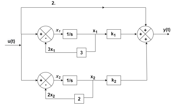
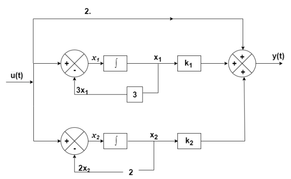
The output equation will be
y(t)=2U+k1x1+k2x2
y=[-88 88] +[2]u
+[2]u
The output equation will be
 =u(t)-3x1
 =-3x1+u(t)
 =-2x2+u(t)
Therefore, the state equation is given as
 =
= +
+
A=
B=
b) By signal flow graph
The transfer function id given as
T= 
Limitations:
1)  =1 for all k
2) All loops should be touching
Number of terms in numerator= Number of forward paths
Number of terms in denominator= Number of loops
Q1) The CLTF T(s)= . Find the state equation?
Sol: T(s)=
=
P1=2/s
P2=-8/s2
L1=-10/s
L2=-100/s2
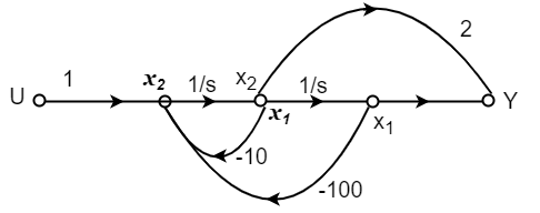
The state equation will be
 =x2
=x2
 =-10x2-100x1+u
 =
= +
+
C) By using differential equation:
Q1) Find the state equation from the given differential equation

Sol: Let y=x1
 =
= =x2
=x2
 =
= =x3
=x3
 =
=
The above differential equation than becomes
 +6
+6 +11x2+6x1=u
 (t) =u-6
 (t)-11x2-6x1
Hence the state equation will be
 =
=  +
+ [u]
[u]
The first order differential equation is given as
 =axx(0)=x0
x(t)= x0=
x0=
Consider state equation
 =Ax(t); x(0)=x0
The solution will be of the form
x(t)=a0+a1t+a2t2+a3t3+….+aiti
Substituting value in above equation
a1+2a2t2+3a3t3+……….=A[a0+a1t+a2t2+a3t3+….+aiti]
a1=Aa0
a2= Aa1=
Aa1= A2a0
A2a0
ai= Aia0
Aia0
Solution for x(t) will be
x(t)=[I+At+ A2t2+………+
 Aiti]x0
The matrix exponential form can be written as

The solution x(t) will be x(t)= x0
x0
 =Ax(t)+Bu(t) and x(0)=x0
 - Ax(t)=Bu(t)
Multiplying both sides by 
 [
[ - Ax(t)]=
 =
= Bu(t)
Bu(t)
Integrating both sides w.r.t t we get
 =
=  d
d
 =
= d
d
Multiplying both sides by 
x(t)= x(0)+
x(0)+ d
d
 x(0) is called as Homogeneous solution
 d
d is the Forced solution
At t=t0
x(t)= x(t0)+
 d
d
The above equation is the required solution.
Solution of non-homogeneous state equation
Let the scalar state equation be
 =ax+bu
 -ax=bu
Multiplying both sides by e-at
x(t) =eatx(0)+ d
d
Then for non-homogeneous state equation
 =Ax+Bu
The solution x(t) can be given as
x(t) =eAtx(0)+ d
d
The above equation is the required solution.
Controllability: A control system is said to be completely controllable if it’s possible to transfer the state of system from initial state to any other required state.
[S]= [B AB AB2 AB3 ------------------- An-1B]
Kalman’s Test: A system is said to be completely controllable if determinant of matrix is not equal to zero, or the rank of the following matrix should be to ‘n’.
n---- order of the matrix.
If  ≠0 then completely controllable
If  =0 then not controllable
Question: A system is represented by following state model A=  B=
B= find whether it is controllable or not?
Solution: A=  B=
B=
So order of matrix is n=2
[S]=[B AB]
= 
 =0 hence, system is not controllable.
Observability: A system is said to be completely observable if it is possible to determine the initial state of system by observing the output for finite interval of time.
Calman’s Test: A system is said to be completely observable within the determinant of following matrix is not equal to zero, or, the matrix rank should be equal to 1.
[Q]= [CT ATCT (AT)2CT ----------(AT)n-1CT]
If ≠0 then completely observable
=0 then not observable
Question: A system is represented by following state model A=  B=
B= , C=[1 1] test whether the system is observable or not?
Solution: AT=  CT=
CT=
[Q]=[CT ATCT]
=
=
=
=0
 =0 hence not observable.
Equivalence between transfer function and state variable representations
The state of a system is a minimal set of variables known as state variables. The knowledge of these variables at any instance of time together with the knowledge of the inputs for the same instance of time, determines the complete behaviour of the system. The fewer drawbacks in the transfer function method for representing any system led to the use of state variables in analysis of system. Few advantages are listed below:
- The state space can be used for linear or nonlinear, time-variant or time-invariant systems.
- It is easier to apply where Laplace transform cannot be applied.
- The nth order differential equation can be expressed as 'n' equation of first order.
- It is a time domain method.
- As this is time domain method, therefore this method is suitable for digital computer computation.
- On the basis of the given performance index, this system can be designed for an optimal condition.
Representation of state space: The system shown below has ‘m’ inputs, ‘p, outputs and ‘n’ number of state variables. The state equation gives us the relation between the state variables and the inputs.

So, the above system shown can be described through equations as
 =f1 (x1, x2,…….xn , u1, u2……… ,um)
 =f2 (x1, x2,…….xn , u1, u2……… ,um)
 =f1 (x1, x2,…….xn , u1, u2……… ,um) (1)
The above set of equations can be represented as
 =f(x(t),u(t)) (2)
As we are concerned for time invariant system, for which the term  in (1) is linear combination of state variables and input. So,
 (t)=2tx1+x2+u1+u2 (3)
 =a11x1(t)+a12x2(t)+…a1nxn(t)+b11u1(t)+b12u2(t)+…….+b1mum(t)
 =a21x1(t)+a22x2(t)+…a2nxn(t)+b21u1(t)+b22u2(t)+…….+b2mum(t)
 =an1x1(t)+an2x2(t)+…annxn(t)+bn1u1(t)+bn2u2(t)+…….+bnmum(t)
The above equation can be represented in matrix form as given below
 (4)
(4)
The above coefficients aij and bji in equation (4) can be written in vector matrix form as
 =Ax(t)+Bu(t)(5)
The output of the system can be represented by linear combination of state variables and inputs.
y1=c11x1(t)+c12x2(t)+…….+c1nxn+d11u1+………..+d1mum
y2=c21x1(t)+c22x2(t)+…….+c2nxn+d21u1+………..+d2mum
yr=cr1x1(t)+cr2x2(t)+…….+crnxn+dr1u1+………..+drmum (6)
The equation (6) can be represented in matrix form as  (7)
(7)
Where coefficients cij and dji are constants. The output equation is given as
Y=CX+DU (8)
The above figure shows the state model of a system with two inputs u1(t) and u2(t), and having outputs y1(t) and y2(t). We know that the output equation is given as
Y(t)=Cx(t)+Du(t) (1)
 (2)
(2)
Taking L.T of equation (9)
Y(s)=CX(s)+DU(s) (3)
Taking L.T of equation (10)
SX(s)=AX(s)+BU(s) (12)
X(s)=[SI-A]-1BU(s) (13)
Y(s)=CX(s)+DU(s)
Y(s)=C{[SI-A]-1BU(s)} + DU(s)
 = C{[SI-A]-1B} + D (14)
[SI-A]-1=
The denominator of equation (14) is the characteristic equation
[SI-A]=0
Pole placement design by state variable feedback
The state-space design method is based on the pole-placement method and the quadratic optimal regulator method. The pole placement method is similar to the root-locus method. In that we place closed-loop poles at desired locations. The basic difference is that in the root-locus design we place only the dominant closed loop poles at the desired locations, while in the pole-placement method we place all closed-loop poles at desired locations. The state variable feedback may be used to achieve the desired pole locations of the closed-loop transfer function.The approach is based on the feedback of all the state variables, and therefore u = Kx.When using this state variable feedback, the roots of the characteristic equation are placed where the transient performance meets the desired response.
The nth order state model is given as
 =Ax(t)+Bu(t)
y=Cx
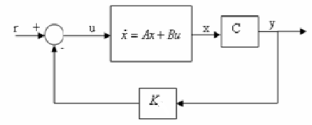
Fig: State variable feedback system
The state variable feedback is given as
 =Kx = [k1 k2 ……….kn]
The block diagram is shown above. From above figure we can write
u = -Kx+r
Where u = Plant input and r = system input
The necessary condition for pole placement is that the system should be completely controllable.
Design steps of pole placement:
- Check the controllability condition for the system. If system is completely controllable then proceed to next step.
- Determine a1,a2 …. an from matrix A using characteristic equation |
 I-A|= sn+a1sn-1+…..+an-1s+an
 - Determine transformation matrix T. By T=QW
Where Q=controllability matrix
W=
4. From the eigenvalues  …….
……. determine the characteristic polynomial (s-
 )(s-
)(s- )….(s-
 )= sn+α1sn-1+…..+ α n-1s+ αn. Then determine α1 ,α2,…….αn
5. Determine the state feedback matrix K , which is given as
K=[αn- anαn-1 an-1 …………..α2 – a2 α1- a1]T-1
Necessity of anobserver
An observer is a dynamic system that is used to estimate the state of a system or some of the states of a system. A full-state observer is used to estimate all the states of the system. The observer can be designed as either a continuous-time system or a discrete-time system. The characteristics are the same, and the design processes are at least very similar and, in some cases, identical. These notes will focus primarily on continuous-time observers.
The purpose of the observer is to generate an estimate of the state x(t) based on measurements of the system output y(t) and the system input u(t). The observer is an nth-order linear dynamic system, where n is the number of state variables in the system.
Design of full order observer
Consider the system defined by
 =Ax(t)+Bu(t)
y=Cx
But for a completely observable system the transformation matrix Q is given as
Q=(WN*)-1
N= [C* A*C* (A*)2C* ----------(A*)n-1C*]
A*=conjugate transpose of A
C*= conjugate transpose of C
W=
Where  …….
……. are coefficients of original state equation
| I-A|= sn+a1sn-1+…..+an-1s+an
Let us consider a new state variable as x=Q
 =Q-1AQ
 +Q-1Bu
y=CQ
Q-1AQ=
Q-1B=
CQ=[0 0 0 …….0 1]
Let the state observer dynamics be

=(A- C)
C) + Bu+
+ Bu+ Cx
Cx
Now,  =Q
=Q
Substituting value of  in
in  we get
 =Q-1((A-
 C)Q
C)Q +Q-1Bu+Q-1
 CQ
CQ
But we also know
 =Q-1AQ
 +Q-1Bu
 -
- = Q-1((A-
 C)Q(
C)Q( -
- )
)
Let  =
= -
-
 = Q-1(A-
 C)Q
C)Q
The main requirement here is to make error dynamics asymptotically stable and  (t) should reach zero. For determining
  we first select the desired observer poles which are the eigenvalues of A-
 C and then finding
  .
.
We also know Q-1=WN*
Q-1 =
=
 =
= 
Q-1 can also be written as
Q-1 =
=
But CQ=[0 0 0……….1]
Q-1 CQ=
CQ=  [0 0 0……….1]=
The characteristic equation is given as
|sI-Q-1(A- C)Q|=0
sn+(a1+ )sn-1+(a2+
 )sn-2+……+(an+
 =0
=0
Let the desired characteristics equation for the error dynamics be
(s- )(s-
)(s- ………(s-
 =sn+(
=sn+( )sn-1+(
 2)sn-2+……+(
 n
n =0
=0
a1+ =
=
.
.
.
an+ =
= n
n
Hence Q-1 =
= =
=
 =Q
=Q
=(WN*)-1
Once the desired eigenvalues are selected the full order state observer can be designed, provided the system is completely observable.
Q) Consider a system  =Ax(t)+Bu(t)
y=Cx
Where A= B=
B= C=[0 1]. Design a full order stet observer, assuming that eigenvalues of the observer matrix are
  =-1.8+j2.4 and
  =-1.8-j2.4?
Sol: The characteristic equation of the system is given as
|sI-A|= =s2-20.6=s2+a1s+a2=0
a1=0
a2=-20.6
The desired characteristic equation is given as
(s- )(s-
)(s- ………(s-
 =(s+1.8+j2.4)(s+1.8-j2.4)=s2+3.6s+9=s2+a1s+a2=0
a1=3.6
a2=9
The observer gain matrix  is given as
 =(WN*)-1
For above case we can write
 =(WN*)-1
 =
= =
=