Unit 1

SETS

1.1             Set and Set Operations

A set is a group or collection of objects or numbers, considered as an entity unto itself. Sets are usually symbolized by uppercase, italicized, boldface letters such as A, B, S, or Z. Each object or number in a set is called a member or element of the set.

Examples include the set of all computers in the world, the set of all apples on a tree, and the set of all irrational numbers between 0 and 1.

Set Operations

The union of two sets is a set containing all elements that are in A or in B (possibly both).

For example, {1,2}∪{2,3}={1,2,3}.

Thus, we can write x∈(A∪B) if and only if (x∈A) or (x∈B).

Note that A∪B=B∪A.

In Figure the union of sets A and B is shown by the shaded area in the Venn diagram.

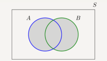
The shaded area shows the set B U A

The intersection of two sets A and B, denoted by A∩B, consists of all elements that are both in A andB.

For example, {1,2}∩{2,3}={2}.

In Figure the intersection of sets A and B is shown by the shaded area using a Venn diagram.

     The shaded area shows A   B

The complement of a set A, denoted by Ac or A¯, is the set of all elements that are in the universal set S but are not in A. In Figure  A¯ is shown by the shaded area using a Venn diagram.

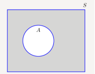
= Ac

The difference is defined as follows. The set A-B consists of elements that are in A but not in B.

For example

If A = {1,2,3}  and B = {3,5}  then A-B = {1,2}

In the figure A-B is shown by shaded area using Venn diagram. A-B = A Bc

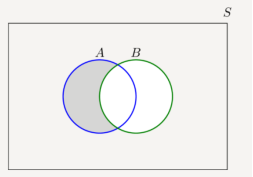
The shaded area shows A-B

Two sets A and B are mutually exclusive or disjoint if they do not have any shared elements, i.e., their intersection is the empty set, A∩B=∅. More generally, several sets are called disjoint if they are pairwise disjoint, i.e., no two of them share a commonelement. Figure shows three disjoint sets.

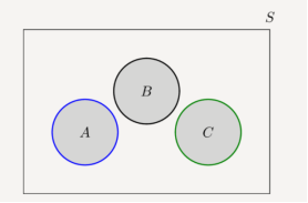
A , B and C are disjoints

De Morgan's law

For any sets A1, A2, ⋯, An, we have

(A1∪A2∪A3∪⋯An)c=A1c1∩A2c∩A3c⋯∩Anc.

(A1∩A2∩A3∩⋯An)c=A1c∪A2c∪A3c⋯∪Anc.

Distributive law

For any sets A, B, and C we have

A∩(B∪C)=(A∩B)∪(A∩C);

A∪(B∩C)=(A∪B)∩(A∪C).

If the universal set is given by S = {1,2,3,4,5,6}

A={1,2}  B={2,4,5}  C ={1,5,6} are three sets find the following sets :

a)     A U B

b)    A B

c)     A -

d)    B -

e)     Checking De Morgan’s law by finding (AUB) c   and A cBc

f)       Check Distributive law find A (B C) and (A B) (A C)

Solution:

a)     A U B = { 1,2,4,5}

b)    A B = {2}

c)       = { 3,4,5,6}  (    consists of elements that are in S but not in A)

d)       = {1,3,6}

e)     We have 

(AUB) c   = {1,2,4,5} c   = { 3,6}

Which is the same as

A c B c = {3,4,5,6}   {1,3,6}

f)       We have (A   (B   C) ) = {1,2} {1,2,3,4,5,6} = {1,2}

(A B) (A   C) = {2} {1} = {1,2}

1.2 Probability Space:

The mathematical concept of a probability space, which has three components (Ω, B, P), respectively the sample space, event space, and probability function.

Ω: sample space. Set of outcomes of an experiment.

Example: tossing a coin twice.

Ω = {HH, HT, T T, T H}

An event is a subset of Ω.

Examples:

(i)                “at least one head” is {HH, HT, T H};

(ii)             “no more than one head” is {HT, T H, T T}. &etc.

In probability theory, the event space B is modelled as a σ-algebra (or σ-field) of Ω, which is a collection of subsets of Ω with the following properties:

(1) ∅∈ B

(2) If an event A ∈ B, then Ac ∈ B (closed under complementation)

(3) If A1, A2, . . . ∈ B, then ∪ ∞ i=1Ai ∈ B (closed under countable union).

A countable sequence can be indexed using the natural integers.

Consider the two-coin toss. Even for this simple sample space

Ω = {HH, HT, T T, T H},

There are multiple σ-algebras:

1. {∅, Ω}: “trivial”σ-algebra

2. The “powerset” P(Ω), which contains all the subsets of Ω

Finally, a probability function P assigns a number (“probability”) to each event in B.

It is a function mapping B → [0, 1] satisfying:

1. P(A) ≥ 0, for all A ∈ B.

2. P(Ω) = 1

3. Countable additivity: If A1, A2, ···∈ B are pairwise disjoint (i.e., Ai ∩Aj = ∅, for all i 6= j), then P(∪ ∞ i=1Ai) = P∞ i=1 P(Ai).

Define: Support of P is the set {A ∈B : P(A) > 0}.

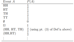
Example: Return to 2-coin toss. Assuming that the coin is fair (50/50 chance of getting heads/tails), then the probability function for the σ-algebra consisting of all subsets of Ω is

1.3 Conditional Probability and Bayes Theorem

Conditional probabilities arise naturally in the investigation of experiments where an outcome of  trial affect the outcomes of the subsequent trials.

We try to calculate the probability of the second event (event B) given that the first event (event A) has already happened. If the probability of the event changes when we take the first event into consideration, we can safely say that the probability of event B is dependent of the occurrence of event A.

For example

• Drawing a second ace from a deck given we got the first ace
• Finding the probability of having a disease given you were tested positive
• Finding the probability of liking Harry Potter given we know the person likes fiction

Here there are 2 events:

• Event A is the probability of the event we are trying to calculate.
• Event B is the condition that we know or the event that has happened.

Hence we write the conditional probability as    P ( A/B) , the probability of the occurrence of event A given that B has already happened.

P(A/B) = P( A and B) / P(B) = Probability of occurrence of both A and B / Probability of B

Suppose you draw two cards from a deck and you win if you get a jack followed by an ace (without replacement). What is the probability of winning, given we know that you got a jack in the first turn?

Let event A be getting a jack in the first turn

Let event B be getting an ace in the second turn.

We need to find P(B/A)

P(A) = 4/52

P(B) = 4/51 {no replacement}

P(A and B) = 4/52*4/51= 0.006

P(B/A) = P( A and B)/ P(A) = 0.006/0.077 = 0.078

Here we are determining the probabilities when we know some conditions instead of calculating random probabilities

Bayes Theorem:

The Bayes theorem describes the probability of an event based on the prior knowledge of the conditions that might be related to the event.

If we know the conditional probability  P(A/B) , we can use the bayes rule to find out the reverse probabilities P(B/A).

How can we do that?

P(A/B) = P ( A B) / P(B)

P(B/A) = P ( A B) / P(A)

P ( A B) = P(A/B) * P(B) = P(B/A) * P(A)

P(B/A) = P(A/B) * P(B)/ P(A)

The above statement is the general representation of the Bayes rule.

Example

Rahul’s favourite breakfast is bagels and his favourite lunch is pizza. The probability of Rahul having bagels for breakfast is 0.6. The probability of him having pizza for lunch is 0.5. The probability of him, having a bagel for breakfast given that he eats a pizza for lunch is 0.7.

To calculate the probability of having a pizza for lunch provided you had a bagel for breakfast would be = 0.7 * 0.5/0.6.

1.4 Combinational Probability and Sampling methods

Combinational Probability is the probability of selecting more than one item® from a set of items.

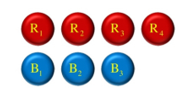
Suppose a box contains 4 red and 3 blue balls. Find the probability of selecting 2 red balls.

n C r  =n! / r! (n-r) !

Solution:

The no of combinations outcomes in selecting two red balls = 4 C 2

Total possible outcomes = 7 C 2

P (Selecting 2 red balls) = 4 C 2/ 7 C 2

=4!/ 2 ! (4-2)! / 7!/ 2! (7-2)! =

4x 3 x 2 x1 / 2x1x2x1/ 7 x 6x4x3x2x1/2x1x5x4x3x2x1= 6/21 = 2/7

Sampling Methods

In a statistical study, sampling methods refer to how we select members from the population to be in the study.Samples can be divided based on following criteria.

• Probability samples - In such samples, each population element has a known probability or chance of being chosen for the sample.
• Non-probability samples - In such samples, one cannot be assured of having known probability of each population element.

Probability sampling methods

Probability sampling methods ensures that the sample chosen represent the population correctly and the survey conducted will be statistically valid. Following are the types of probability sampling methods:

• Simple random sampling. - This method refers to a method having following properties:
  • The population have N objects.
  • The sample have n objects.
  • All possible samples of n objects have equal probability of occurrence.

One example of simple random sampling is lottery method. Assign each population element a unique number and place the numbers in bowl.Mix the numbers thoroughly. A blind-folded researcher is to select n numbers. Include those population element in the sample whose number has been selected.

• Stratified sampling - In this type of sampling method, population is divided into groups called strata based on certain common characteristic like geography. Then samples are selected from each group using simple random sampling method and then survey is conducted on people of those samples.
• Cluster sampling - In this type of sampling method, each population member is assigned to a unique group called cluster. A sample cluster is selected using simple random sampling method and then survey is conducted on people of that sample cluster.
• Multistage sampling - In such case, combination of different sampling methods at different stages. For example, at first stage, cluster sampling can be used to choose clusters from population and then sample random sampling can be used to choose elements from each cluster for the final sample.
• Systematic random sampling - In this type of sampling method, a list of every member of population is created and then first sample element is randomly selected from first k elements. Thereafter, every kth element is selected from the list.

Non-probability sampling methods

Non-probability sampling methods are convenient and cost-savvy. But they do not allow to estimate the extent to which sample statistics are likely to vary from population parameters. Whereas probability sampling methods allows that kind of analysis. Following are the types of non-probability sampling methods:

• Voluntary sample - In such sampling methods, interested people are asked to get involved in a voluntary survey. A good example of voluntary sample in on-line poll of a news show where viewers are asked to participate. In voluntary sample, viewers choose the sample, not the one who conducts survey.
• Convenience sample - In such sampling methods, surveyor picks people who are easily available to give their inputs. For example, a surveyer chooses a cinema hall to survey movie viewers. If the cinema hall was selected on the basis that it was easier to reach then it is a convenience sampling method.

References