Unit - 3
Discrete Fourier Transform
We first transform the image to its frequency distribution. Then our black box system performs whatever processing it has to performed, and the output of the black box in this case is not an image, but a transformation. After performing inverse transformation, it is converted into an image which is then viewed in spatial domain.
A signal can be converted from time domain into frequency domain using mathematical operators called transforms. There are many kinds of transformation that does this. Some of them are given below.
- Fourier Series
- Fourier transformation
- Laplace Transform
- Z Transform
Fourier series simply states that, periodic signals can be represented into sum of sines and cosines when multiplied with a certain weight.It further states that periodic signals can be broken down into further signals with the following properties.
- The signals are sines and cosines
- The signals are harmonics of each other
The Fourier Series is given by
The inverse is given by
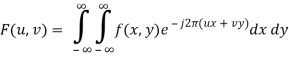
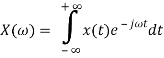
The Fourier transform simply states that that the non-periodic signals whose area under the curve is finite can also be represented into integrals of the sines and cosines after being multiplied by a certain weight. The Fourier transform is given by
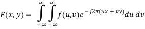
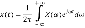
The inverse is given as
The Fourier transform has many wide applications that include, image compression (e.g JPEG compression), filtering and image analysis.
Key takeaway
The Fourier transform is given by

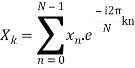
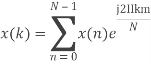
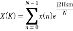
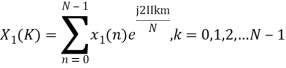
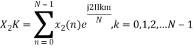
The discrete Fourier transform transforms a sequence of N complex numbers 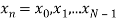 into another sequence of complex numbers
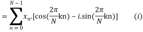
 which is defined by
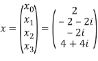
Example:
Let N =4 and
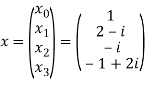
Here we demonstrate how to calculate the DFT of x using equation (1)


Linear Property
If x(t) -> X(w)
Y(t) -> Y(w) then
a x(t) + b y(t) -> a X(w) +b Y(w)
Time Shifting Property
If x(t)⟷F.TX(ω)
Then Time shifting property states that
x(t−t0)⟷F.T e−jω0t X(ω)
Frequency Shifting Property
If x(t)⟷X(ω)
Then frequency shifting property states that
Ejω0t.x(t)⟷X(ω−ω0)
Time Reversal Property
If x(t)⟷X(ω)
Then Time reversal property states that
x(−t)⟷X(−ω)
Differentiation Property
If x(t)⟷X(ω)
Then Differentiation property states that
Dx(t)dt⟷jω.X(ω)
dnx(t)dtn⟷(jω)n.X(ω)
Integration Property
Integration property states that
∫x(t)dt⟷1jω X(ω)
Then
∭...∫x(t)dt⟷(jω)n X(ω)
Multiplication and Convolution Properties
If x(t)⟷X(ω)
y(t)⟷Y(ω)
Then multiplication property states that
x(t).y(t)⟷X(ω)∗Y(ω)
And convolution property states that
x(t)∗y(t)⟷1/2πX(ω).Y(ω)
Key takeaway
Property | Time domain | Frequency Domain |
1. Linearity | Ax1[n] + bx2[n] | AX1[k] + bX2[k] |
2. Time-shifting | x[n - m] | e-j2πkmX(k) |
3. Frequency-shifting (modulation) | e-j2πk0n/Nx[n] | x(k - k0) |
4. Time reversal | x[-n] | X(-k) |
5. Conjugation | x*[n] | X*(-k) |
6. Time-convolution | x1[n]x2[n] |  |
8. Parseval's relation |  |  |
Examples
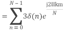
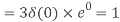
Compute the N-point DFT of x(n)=3δ(n).
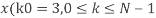
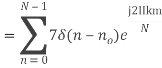
Compute the N-point DFT of x(n)=7(n−n0)
Solution − We know that,
Substituting the value of x(n),
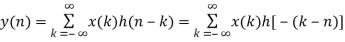
Linear Convolution states that
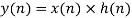
y(n) = x(n) * h(n)

Example 1: h(n) = { 1 , 2 , 1, -1 } & x(n) = { 1, 2, 3, 1 } Find y(n).
METHOD 1: GRAPHICAL REPRESENTATION
Step 1) Find the value of n = nx+ nh = -1 (Starting Index of x(n)+ starting index of h(n))
Step 2) y(n)= { y(-1) , y(0) , y(1), y(2), ….} It goes up to length(xn)+ length(yn) -1. i.e n=-1


METHOD 2: MATHEMATICAL FORMULA
Use Convolution formula
k= 0 to 3 (start index to end index of x(n))
y(n) = x(0) h(n) + x(1) h(n-1) + x(2) h(n-2) + x(3) h(n-3)
METHOD 3: VECTOR FORM (TABULATION METHOD)
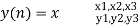
X(n)= {x1,x2,x3} & h(n) ={ h1,h2,h3}
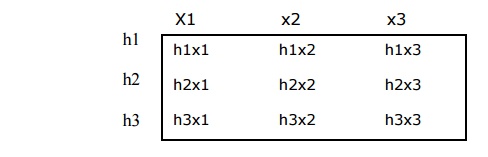
y(-1) = h1 x1
y(0) = h2 x1 + h1 x2
y(1) = h1 x3 + h2x2 + h3 x1 …………
METHOD 4: SIMPLE MULTIPLICATION FORM

Circular convolution
Let us take two finite duration sequences  ,having integer length as N. Their DI are
  reapectively which is shown below
Now we will try to find the DFT of another sequence  , which is given by
By taking the IDFT of the above we get
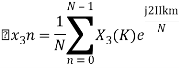
After solving the above equation finally we get

Methods of Circular Convolution
Generally, there are two methods, which are adopted to perform circular convolution and they are −
- Concentric circle method
- Matrix multiplication method
Concentric Circle Method
Let x1(n) and x2(n) be two given sequences. The steps followed for circular convolution of x1(n) and x2(n) are
- Take two concentric circles. Plot N samples of x1(n) on the circumference of the outer circle maintaining equal distance successive points maintaining equal distance successive points in anti-clockwise direction.
- For plotting x2(n), plot N samples of x2(n) in clockwise direction on the inner circle, starting sample placed at the same point as 0th sample of x1(n)
- Multiply corresponding samples on the two circles and add them to get output.
- Rotate the inner circle anti-clockwise with one sample at a time.
Matrix Multiplication Method
Matrix method represents the two given sequence x1(n) and x2(n) in matrix form.
- One of the given sequences is repeated via circular shift of one sample at a time to form a N X N matrix.
- The other sequence is represented as column matrix.
- The multiplication of two matrices give the result of circular convolution.
Key takeaway
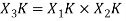
y(n) = x(n) * h(n)

Examples
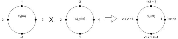
Perform circular convolution of the two sequences, x1(n)= {2,1,2,-1} and x2(n)= {1,2,3,4}
Sol:
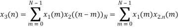
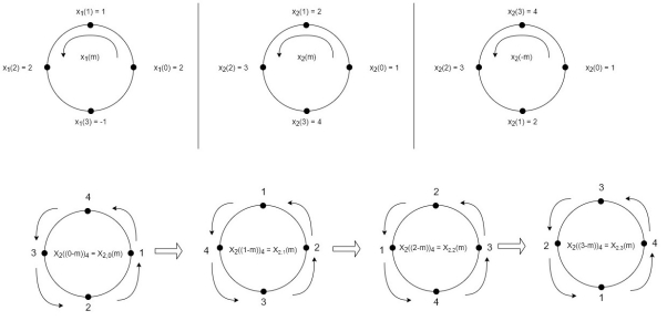
Fig 1 Circular Convolution of x1(n)= {2,1,2,-1} and x2(n)= {1,2,3,4}
(2)
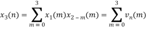
When n=0;
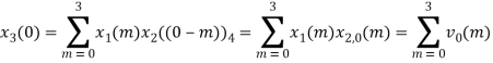
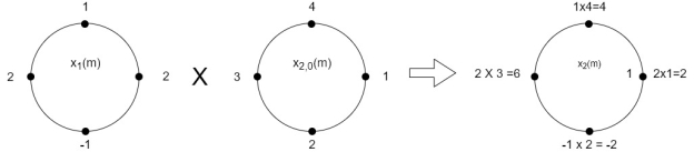
The sum of samples of v0(m) gives x3(0)
⸫ x3(0)=2+4+6-2=10
When n=1;

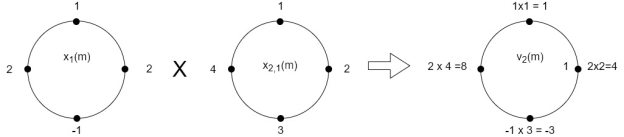
The sum of samples of v1(m) gives x2(1)
⸫ x3(1)=4 + 1 +8-3=10
(3) When n=2;
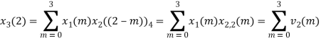

The sum of samples of v2(m) gives x3(2)
⸫ x3(2)=6+2+2-4=6
(4) When n=3;
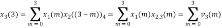
The sum of samples of v3(m) gives x3(3)
⸫ x3(3)=8+ 3+ 4-1= 14
x3(n)={10,10,6,14}
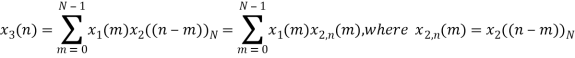
= x1(0) x x2,0(0) + x1(1) x2,0(1) + x1(2) x2,0(2) + x1(3) x2,0(3)
= 2 x 1 + 1 x 4 + 2 x 3 + (-1) x 2 = 2 +4 +6 -2 =10
Certain algorithms permit implementations of Discrete Fourier transform with considerable savings in computation time. These algorithms are known as Fast Fourier Transform.
FFT algorithm are based on fundamental principle of decomposing the computation of DFT of sequence length into successively smaller discrete Fourier transforms.
They are basically two classes of FFT algorithms
- Decimation in time
- Decimation in frequency
Decimation-in-time algorithm
This algorithm is known as Radix-2 DIT-FFT algorithm which means the number of output points N can be expressed as a power of 2 that is N = 2M where M is an integer.
Let x(n) be a sequence where N is assumed to be a power of 2. Decimate or break this sequence into two sequences of length N/2 where one sequence consists of even-indexed values of x(n) and the other of odd-indexed values of x(n).
Xe(n) = x(2n) n= 0,1,……….. N/2-1
Xo(n) = x(2n+1) n= 0,1,……….. N/2 -1
The N-pt DFT of x(n) can be written as
X(k) =  WNnk where k=0,1……….. N-1.
Separating x(n) into even and odd indexed values of x(n) we obtain
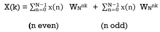
=  WN2nk +
  WN(2n+1)k
=  WN2nk + Wnk
 W N2nk
X(k) =  WN2nk + Wnk
 W N2nk
WN2 =( e-j2π/N) 2 =e-j2π/N/2 = W N/2 .
WN2 = W N/2
X(k) =  W N/2nk + WNk
 WN/2kn
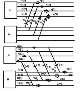
Fig 2 Decimation in time algorithm
W84 = -1
W85 = - W 81
W86 = - W82
W87 = - W83
G(0) – H(0) = x(4)
G(1) - W 81 H(1) = x(5)
G(2) - W82 H(2) = x(6)
G(3) - W83 H(3) = x(7)
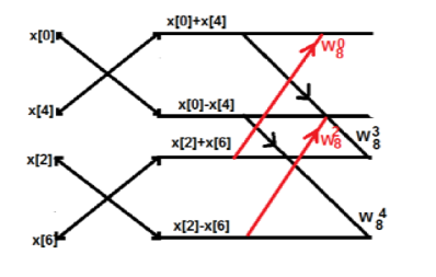
Fig 3 Butterfly Diagram to find W08-W38
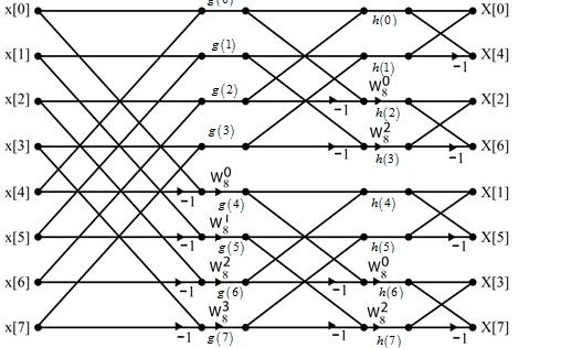
Consider the sequence x[n]={ 2,1,-1,-3,0,1,2,1}. Calculate the FFT.
Arrange the sequence as x(0) x(4) x(2) x(6) x(1) x(5) x(3) x(7)
Since N=8 find the values W80 to W 87
Apply the butterfly diagram to obtain the values.
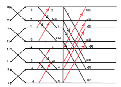
Fig 4 Butterfly Diagram
Decimation in Frequency FFT
Apart from time sequence, an N-point sequence can also be represented in frequency. Let us take a four-point sequence to understand it better.
Let the sequence be x[0],x[1],x[2],x[3]………..x[7]
Mathematically, this sequence can be written as;
X(k) =  WNn-k where k=0,1……….. N-1.
Now let us make one group of sequence number 0 to 3 and another group of sequence 4 to 7. Now, mathematically this can be shown as
=  WNnk +
  WN nk
WN nk
Let us replace n by r, where r = 0, 1 , 2….N/2−1.
=  W N/2nr
We take the first four points x[0],x[1],x[2],x[3] initially, and try to represent them mathematically as follows –
 W 8 nk +
  W8(n+4) k
=  +
+  W8(n+4) k
=  + {
+ {  W8(4) k } W8nk
X[0] =  + X[n+4]
X[1] =  + X[n+4]) W8nk
= X(0) – X(4) + (x[1] – X[5]) W81 + ( X[2] – X[6] )W82 + X(3) – X(7) W83
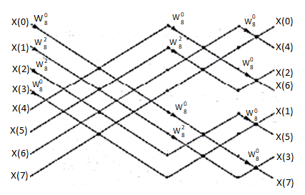
Fig 5 DIF –FFT Algorithm
Find the DIF –FFT of the sequence x(n)= { 1,-1,-1,1,1,1,-1} using Dif-FFT algorithm.
X(0)= 20X(4) =0
X(1) = -5.828- j2.414X(5) = -0.1716 + j 0.4141
X(2) = 0X(6) = 0
X(3) = -0.171 – j 0.4142X(7) = -5.8284 + j2.4142
Key takeaway
The N-pt DFT of x(n) can be written as
X(k) =  WNnk where k=0,1……….. N-1.
The below give equation is called as Plancherel’s formula
 (1)
(1)
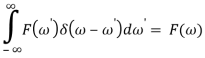
The integral of delta function is given as shown below
 (2)
(2)
The inverse Fourier transform is shown as
 (3)
(3)
From 1 can write
 (4)
(4)
Rearranging the above equation we have
 (5)
(5)
Use delta- fn here
The integral representation of  function in 2 is
 (6)
(6)
 (7)
(7)
The equation 7 is obtained because of the  function property shown below
The Parseval’s Theorem is given below
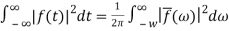 (8)
(8)
The basic realization techniques used for filters are direct form, cascade form and parallel form. In this section we will study all in detail. This section overviews ability to implement finite impulse response (FIR) and infinite impulse response (IIR) filters using different structures in terms of block diagram and signal flow graph.
For an LTI system the transfer function is given as
H(z)=  (1)
(1)
The difference equation can be written as
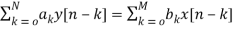 (2)
(2)
x(n)= system input
y(n)=system output
When a0≠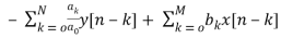 (3)
(3)
The above equation implementation requires some basic blocks shown below
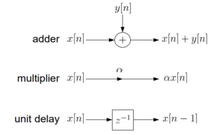
Fig 6 Block diagram representation
Example: The above blocks can be easily understood with the help of one example. For the standard LTI system with difference equation
Y[n]=-a1y[n-1]-a2y[n-2]+b0x[n]. Draw the block diagram for the given equation.
Sol: We already know that x[n] and y[n] are the input and output to the system respectively.
- If we need the term y[n-1] we need a delay block after y[n], and one more delay block after y[n-1] to get y[n-2].
- For getting term -a1y[n-1] we need multiplier of -a1and same for -a2.
- To get complete term -a1y[n-1]-a2y[n-2]+b0x[n] we need adders so that the we get the final equation.
- The final figure using 2 adders, 3 multipliers and 2 delay block is shown below.
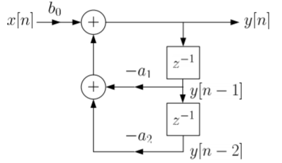
Fig 7: Block diagram representation
FIR FILTER:
The standard equation for representing the FIR filter is shown below
H(z)= (4)
(4)
From equation (1) and (4) we can conclude that FIR filters do not contain any pole. The difference equation will be
Y[n]=  (5)
(5)
a) Direct Form:
The direct form is directly derived from the difference equation. It can be represented as
y[n]=  (6)
(6)
Where h(k) is the system impulse response.
Expanding the above equation, we get
Y[n]= =h[0]x[n]+h[1]x[n-1]+……h[M]x[n-M] (7)
The block diagram representation for above direct form is shown below.
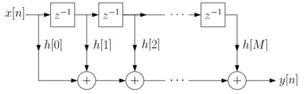
Fig 8: Direct form realization of Fir filter
b) Cascade Form:
As we already know H(z)=
The above equation can be represented as a product of second order polynomial as
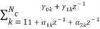
H(z)= =
= (8)
(8)
Mc=|(M+1)/2|
The above equation can be further simplified with intermediate output of system 1 w1(n) fed to the input of second cascade structure and so on.
The difference equation is given as
w1(n)=  +
+ (9)
(9)
w2(n)= 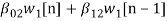 +
+ (10)
(10)
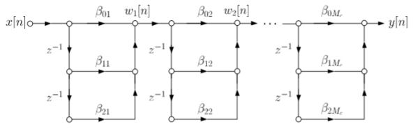
Fig 9: Cascade form FIR filter
IIR FILTER:
The transfer function of IIR filter is given as
H(z)=  (11)
(11)
From above equation we can conclude that an IIR filter contains at least one pole.
a) Direct Form:
The direct form is realised directly from its difference equation
v[n]=  (12)
(12)
y[n]=-  +v[n] (13)
Another way to obtain direct form is by decomposing H(z) into two transfer functions
H(z)=H1(Z). H2(z)
H1(Z)=  (14)
(14)
H2(z)=  (15)
(15)
V(z)=X(z). H1(Z)=X(z) (16)
(16)
Y(z)=V(z). H2(z)=V(z) (17)
(17)
The final realisation block diagram representation of direct form for IIR filter is shown below
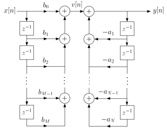
Fig 10: Direct Form realization of IIR Filter
b) Cascade form:
To find the transfer function for cascade for we need to factorize the numerator and denominator polynomials in terms of second order polynomial.
H(z)= =
= (18)
(18)
Nc=|(N+1)/2|
Let us consider M=N=4. Then the cascade realisation for IIR filter is shown below.
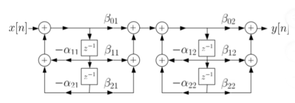
Fig 11: Cascade Form realisation of IIR Filter
Que) For the following LTI system H(z)=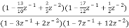 . Realise the cascade form IIR filter.
Sol: H(z)=
The above function can be simplified as
H(z)=
Hence, using the above structure and placing the values of  …. And similarly,
c) Parallel form:
The parallel form is given as H(z)= +
+ (19)
(19)
Nc=(N=2)/2
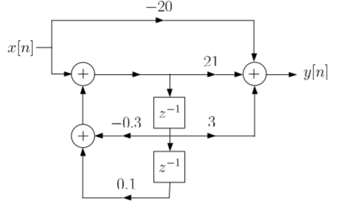
Que) Draw block diagram for the function using parallel form H(z)=
Sol: H(z)=
Writing above transfer function in standard form for parallel realisation we get
H(z)=-20+
The structure is shown below
Key takeaway
Sr No | FIR Digital Filter | IIR Digital Filter |
1 | FIR system has finite duration unit sample response. i.e h(n) = 0 for n<0 and n≥M. Thus the unit sample response exists for the duration from 0 to M-1. | IIR system has infinite duration unit sample response i.e h(n) = 0 for n<0. Thus the unit sample response exists for the duration from 0 to ∞. |
2 | FIR systems are non recursive. Thus output of FIR filter depends upon present and past inputs. | IIR systems are recursive. Thus they use feedback. Thus output of IIR filter depends upon present and past inputs as well as past outputs. |
3 | Difference equation of the LSI system for FIR filters becomes 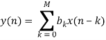 | Difference equation of the LSI system for IIR filters becomes  |
4 | FIR systems has limited or finite memory | IIR system requires infinite memory. |
References:
1. S. K. Mitra, “Digital Signal Processing: A computer based approach”, McGraw Hill, 2011.
2. A.V. Oppenheim and R. W. Schafer, “Discrete Time Signal Processing”, Prentice Hall, 1989.
3. J. G. Proakis and D.G. Manolakis, “Digital Signal Processing: Principles, Algorithms And Applications”, Prentice Hall, 1997.
4. L. R. Rabiner and B. Gold, “Theory and Application of Digital Signal Processing”, Prentice Hall, 1992.
5. J. R. Johnson, “Introduction to Digital Signal Processing”, Prentice Hall, 1992.
6. D. J. DeFatta, J. G. Lucas andW. S. Hodgkiss, “Digital Signal Processing”, John Wiley & Sons,1988.


