Unit 1

Signals

1.1 Introduction

Definition: A signal is defined as a physical quantity that varies with time, space, or any other independent variable.

The signal may depend on one or more independent variables. If the signal depends on one variable, then it is known as a one-dimensional signal. If it depends on two independent variables, then the signal is known as a two-dimensional signal. Examples are pictures, X-ray images, and sonograms.

The multidimensional signal depends on many variables.

Graphical, Functional, Tabular and Sequence Representation of Discrete-time Signal

1. Graphical Representation

Let us consider a signal x(n) with values x(0) =2; x(1)=1.5;x(1)=2;x(3)=1.5

The discrete-time signal can be represented graphically as:

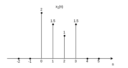
Figure 1. Discrete-time in graphical

2.     Functional Representation

The discrete time signal as shown in figure can be represented using functional representation as below:

x(n) =             2     for n=0

x = 1.5 for n=1

1     for n=2

x =1.5 for n=3

Tabular Representation

The discrete-time signal can also be represented as:

Sequence Representation

A finite duration sequence with time origin (n=0) indicated by the symbol is represented as

x(n) = {1, 2, 2, 0.5, 1.5}

A finite duration sequence can be represented as

x(n) = {……. 0.2, 1, -1, 3, 2……….}

A finite duration sequence that satisfies the condition x(n) =0 for n<0 can be represented as

x(n)={2, 4, 6, 8, -3}

Graphical, Functional, Tabular and Sequence Representation of continuous-time Signal

Graphical Representation

Many phenomena in our physical world are described in terms of continuous-time signals. Some examples of continuous-time signals include voltage or current waveforms in an electronic circuit;

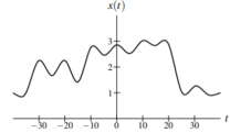
Figure 2. Discrete-time in graphical

Key Take-Aways:

1. Definition of signal
2. Representation of signal in discrete time
3. Representation of signal in continuous time

1.2 Basics of Elementary Signals

      Elementary continuous-time signals

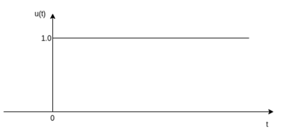
1. Unit step function

The unit step sequence is defined as:

u(t) = 1 for t

= 0 for t<0

From the above equation, we find the when the argument t in u(t) is less than zero then the unit step function is zero and when the argument t in u(t) is greater than or equal to zero then the unit step function is unity

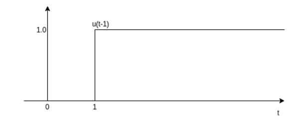
Similarly, for a shifted unit step function u(t-a) is zero if the argument (t-a) <0 or t<a and is one of the argument (t-a) > 0 or t>a.

That is

u(t-a) = 1  for  t>a

=0    for t<a

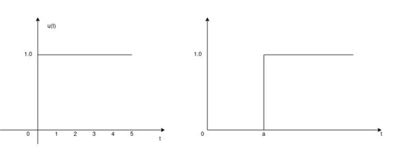
Figure 3. Unit step function

Unit ramp function

The unit ramp function is defined as:

r(t) = t    for t

=0    for t<0

Or

r(t) = t u(t)

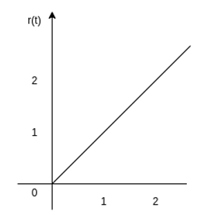
Figure 4. Unit ramp function

The ramp function can be obtained by applying the unit step function to an integrator.

r(t) = dt =    ( in the time interval t>0)

The unit step function can be obtained by differentiating the unit ramp function

Thus

u(t) = d/dt r(t)

Unit parabolic function

The unit parabolic function is given by

p(t) = t 2 / 2      for t 0

= 0          for t<0

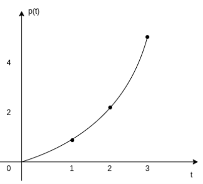
Figure 5. Unit parabolic function

Or

p(t) = t2/2 u(t)

Impulse function

The impulse function occupies an important place in signal analysis. It is defined as

dt =1

And

δ(t) =0  for t

The impulse function has zero amplitude everywhere except at t=0. At t=0 the amplitude is infinity such that the area under the curve is equal to one. The unit impulse function can be obtained by using a limiting process on the rectangular pulse as shown in the figure.

Note that the area under the rectangular pulse is equal to unity.

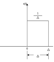
Figure 6. Impulse function

The rectangular pulse function of the figure can be expressed as

x(t) = 1/ ∆ [ u(t) – u(t-∆)] …………………………………..(1)

The impulse function can be obtained when the width ∆ ->0 that is

δ(t) = lim ∆-> 0 x(t)

= lim ∆-> 0 1/ ∆ [ u(t) – u(t-∆)]

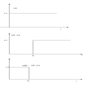
Figure 7. Unit impulse with a delay function

The delayed unit impulse function is defined as

=1     for t=a

And =0    for t a

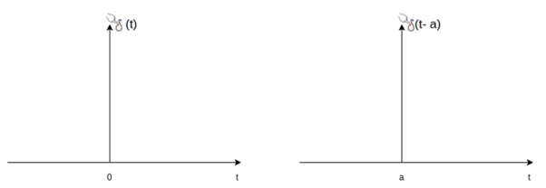
Figure 8. Impulse function

Sinusoidal signal  

A continuous-time sinusoidal signal is given by

x(t) = A sin ( + ) ---------------------------------(1)

Where A is the amplitude, Ω is the frequency in radians per second, and is the phase angle in radians.

The figure shows the waveform of the sinusoidal signal with A=1, = -π/3 with period 2π/Ω.

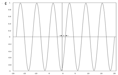
Figure 9. Sinusoidal function

Real exponential and complex exponential

Real exponential

Figure 10. Real exponential function

A real exponential signal is defined as

x(t) = A e at --------------------------------(1)

Where both A and a are real. Depending on the value of ‘a’ we get different signals. If ‘a’ is positive the signal x(t) is growing exponential as shown in fig(b) If ‘a’ is negative then x(t) is decaying exponential as shown in fig(c). For a=0 x(t) is constant.

Complex exponential signal.

The most general for of complex exponential signal is given by

x(t) = e st ---------------------------------------(1)

Where s is a complex variable defined as

s = + j Ω

Therefore

x(t) = e st = e s(+ j Ω) = e t . e j Ωt

Using Euler identity, we can expand

e j Ωt = cos Ω t + j sin Ωt

Substituting in eq(1) we get

x(t) = e t [ cos Ω t + j sin Ω t]

Depending on the values of and Ω we get different signals.

1. If =0 and Ω =0 x(t) = 1 that is the signal x(t) is a pure DC signal.
2. If Ω=0 then s = , x(t) = e t which decays exponentially for <0 and grows exponentially for > 0.
3. If =0 then s= jΩ gives x(t) = e j Ωt a sinusoidal signal with ɸ=0
4. If <0 with finite Ω we get an exponentially decaying sinusoidal signal.
5. If 0 with finite Ω we get an exponentially growing sinusoidal signal.

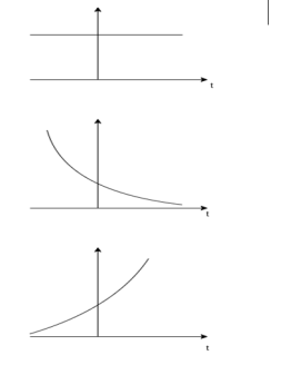
Figure 11. Exponential function fo

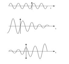
Figure 12. Complex exponential function

Rectangular Pulse:

The rectangular pulse function is defined as

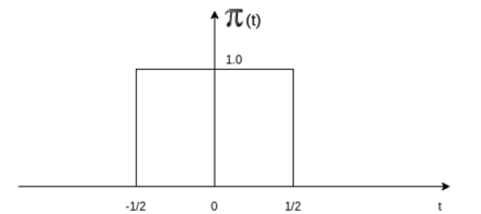
Figure 13. Rectangular pulse

     for |t| ½

=0     otherwise

Triangular pulse function

The unit triangular function is defined as

∆a(t)   =      1 - |t|/a       |t| a

0             |t| a

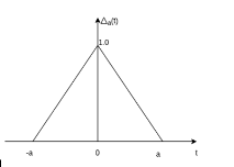
Figure 14. Triangular pulse

Signum function

The sinc function is defined by the expression

Sinc(t) = sin t/t          -∞ < t < ∞

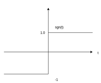
Figure 15. Signum function

The sinc function oscillates with period 2π and decays with increasing t. Its value is zero at nπ, n = ±1, ±2, …………………….. It is an even function of t.

Gaussian function:

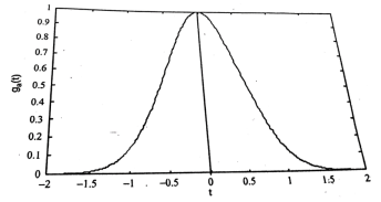
Figure 16. Gaussian function

The Gaussian function is defined by the expression

Ga(t) = e – at ^2  - ∞ <t<∞

This function is extensively used in probability theory.

Problems:

Sketch the continuous-time signal x(t) = 2 sin πt for interval 0 2. Sample the continuous-time signal with a sampling period T =0.2 sec and sketch the discrete-time signal.

Solution:

Given:

x(t) = 2 sin πt

To sketch the signal we have values x(t) for different values of t, that is

x(0) = 2 sin π (0) = 0.

x(0.25) = 2 sin π (0.25) = √2

x(0.5) = 2 sin π (0.5) = 2

x(0.75) = 2 sin π (0.75) = √2.

x(1) = 2 sin π (1) = 0

x(1.25) = 2 sin π (1.25 = -√2

x(1.5) = 2 sin π (1.5) = -2.

x(0.25) = 2 sin π (1.75) = - √2

x(2) = 2 sin 2π =0

Take t on x-axis and x(t) on y-axis. Mark the above points and join all the points by a smooth curve to get continuous signal as shown in fig (a) . Given sampling period T =0.2

Sketch the signal x(t) = e -t for an interval 0 t 2

Sample the signal with a sampling period T=0.2 second and sketch the discrete time signal.

Solution:

Given

x(t) = e -t ; x(0) =1; x(0.5) = 0.606, x(1)= 0.36768; x(1.5) = 0.2237, x(2) = 0.1353

To get signal x(t) mark the above points and draw a smooth curve joining all points as shown in figure (a)

x(nT) = x(t) | t =nT

= x(t) | t=0.2n

x(0.2n) = e -0.2 n

x(0) =1

x(1) = e – 0.2 = 0.818

x(2) = e – 0.4 = 0.67

x(3) = e – 0.6 = 0.5488

x(2) = e – 0.8 = 0.449

x(2) = e – 1 = 0.3678

x(2) = e – 1.2 = 0.3012

x(2) = e – 1.4 = 0.2466

x(2) = e – 1.6 = 0.2022

x(2) = e – 1.8 = 0.1653

x(2) = e – 2 = 0.1353

Evaluate the following integrals:

(i)                – αt 2 δ(t-10) dt

Given

(i)                – αt 2 δ(t-10) dt

From the property

δ(t-to) dt = x(to)

We have

– αt 2 δ(t-10) dt = e – αt2 |t=10

e-100 α

δ(t-10) =1  for t=10

= 0 otherwise

Given

2 δ(t-3) dt = t 2 | t=3  =9

δ(t-3)   = 1  for t=3

=0  otherwise

δ(t) x(t) dt = -dx/dt(0)

Let u=x(t)

Dv = d/dt δ(t)

v = δ(t)

= uv - du

Du = dx/dt

δ(t) x(t) dt = x(t) δ(t) | - ∞ - x(t) δ(t) dt = - dx/dt (0)

Elementary Discrete-Time Signals

Unit step sequence:

The unit step sequence is defined as:

u(n) = 1   for n

=0    for n<0

Figure 17. Unit step in discrete

Unit ramp sequence:

The unit ramp sequence is defined as

r(n) = n for n

=0  for n<0

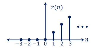
Figure 18. Unit ramp sequence

Unit sample sequence

The unit sample sequence is defined as

for n=0

=0  for n 0

The graphical representation of is shown in the figure.

Figure 19. Unit sample sequence

The unit impulse function has the following properties:

= u(n) – u(n-1)

u(n) =

= (n-no) = x(no)

Exponential sequence

The exponential sequence is a sequence of the form

x(n) = a n for all n.

The figure illustrates the different types of discrete-time exponential signals. When the value of α > 1 the sequence grows exponentially and when the value is 0<a<1 the sequence decay exponentially.

When a<0 the discrete-time signal takes alternating signs.

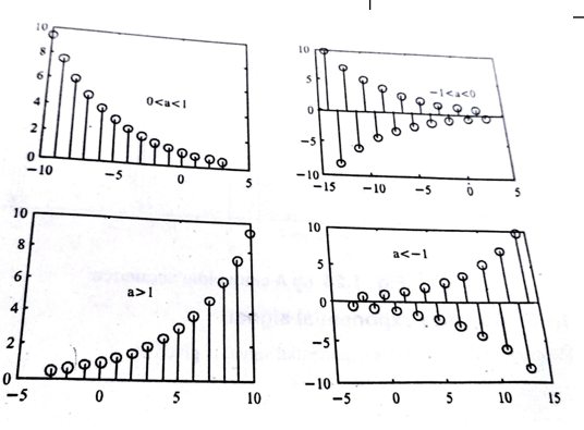
Figure 20. Exponential sequence

Sinusoidal signal

The discrete-time sinusoidal signal is given by

x(n)= A cos (won + ɸ)---------------------------(1)

Where wo is the frequency and ɸ is the phase

Using Euler’s identity we can write

A cos(won + ɸ) = A/2 e jɸ . e j won + A/2 e-jɸ e -jwon ---------------------(2)

Since | e jwon | 2 =1

The energy of the signal is infinite and the average power of the signal is 1.

An example of a discrete-time sinusoidal signal is shown in the figure.

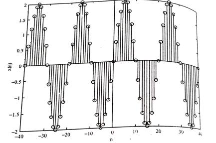
Figure 21. Sinusoidal sequence

Complex exponential signals.

The discrete time complex exponential signal is given by

x(n) = a n e j (won + ɸ) ------------------------------------(1)

= a n cos (wo + ɸ) + j a n sin (won + ɸ) .

For |a| =1 the real and imaginary parts of the complex exponential sequence are sinusoidal.

For |a| < 1 the amplitude of sinusoidal sequence decays exponentially

For |a| > 1 the amplitude of the sinusoidal sequences increases exponentially. Examples of these signals are given in the figure.

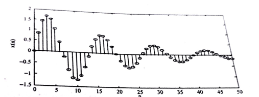
Figure 22. Complex exponential sequence

Key Takeaways

1. Classification of signal in continuous time
2. Classification of signal in discrete time

1.3 Basic Operations on Signals

Time Shifting

Let us consider a signal x(t) as shown in the figure. The time-shifting of x(t) may delay or advance the signal in time. Mathematically this can be represented by

y(t) = x(t-T) ------------------------------------------(1)

If T is positive the shifting delays the signal as shown in the figure.

If T is negative the shifting advances the signal as shown in the figure.

Figure 23. Time Shifting

Similarly, the time-shifting operation of discrete-time signals is represented by

y(n) = x(n-k)

Which shows that the signal y(n) can be obtained by shifting x(n) by k units. If k is positive the shift is to the right (delay) and if k is negative the shift is to the left. Let us consider a signal x(n) as shown in the figure. The signal x(n-2) is obtained by shifting x(n-2) is obtained by shifting x(n) right by 2 units of time. The result is shown in fig (b). On the other hand x(n+3) is obtained by shifting x(n) left by three units of time.

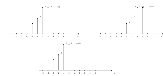
Figure 24. Time-shifting in discrete time

Time Reversal

The time-reversal of signal x(t) can be obtained by folding the signal about t=0. It is denoted by x(-t). The signal x1(t) and its reflection x(-t) are illustrated in fig a and b respectively.

Figure 25. Time Reversal

The signal x(-t+2) is obtained by delaying x1(-t) by two units of time and x1(-t-2) is obtained by advancing x1(-t) by two units of time. The signals x1(-t+2) and x1(-t-2) are shown in figure ( c) and (d).

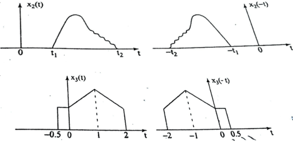
Figure 26. Operation on time reversal

The time-reversal of the discrete-time signal can be obtained by folding the sequence x(n) about n=0. For signal x1(n) in fig, the time-reversal signal x1(-n) is shown in fig (b).

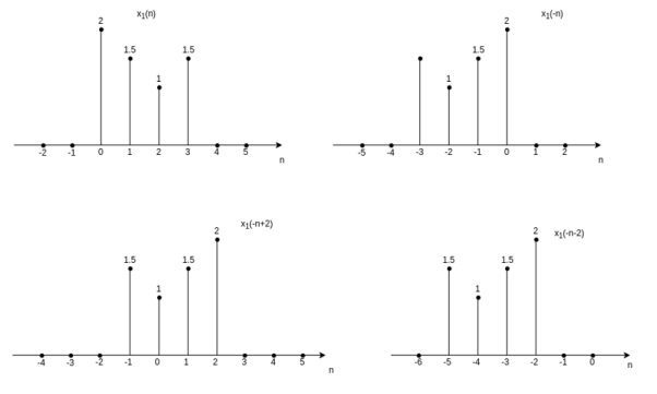
Figure 27. Operation of time reversal in discrete

The signal x1(-n+2) is obtained by delaying x1(-n) by two units of time and x1(-n-2) is obtained by advancing x1(-n) by two units of time. The other examples for time-reversal of the discrete-time signal are obtained by fig (a) and (b).

Figure 28. Input and output signal

Problem:

Sketch the following signals

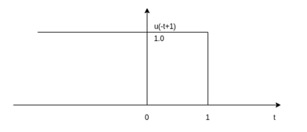
(i)                u(-t+1)

Step 1: draw the unit step signal

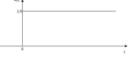
Step 2: Fold the signal about t-0 as shown in fig (b)

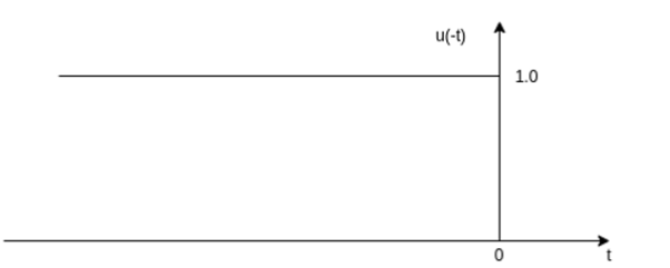
Step 3: Shift the signal u(-t) right by one unit as shown in fig(c )

(ii)              x(t) = -2 u(t-1)

Step 1: Draw the unit step signal

Step 2: Shift the signal u(t) right by one unit of time as shown in the figure.

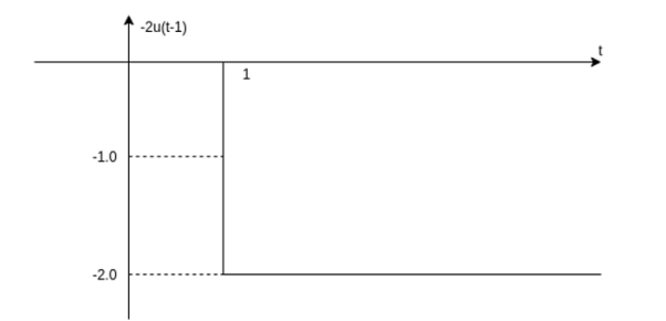
Step3: Multiply the signal u(t-1) with -2

Amplitude Scaling:

Consider a signal x(t) that is fed to an amplifier with a gain of 3 then the output of an amplifier can be represented by

y(t) = 3 x(t)

That is the output y(t) is identical in shape to the input signal x(t) but its amplitude is thrice everywhere. This concept is illustrated in the figure.

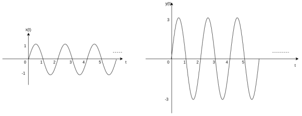
Figure 29. Amplitude Scaling

From fig we find that the amplitude is rescaled hence the name amplitude scaling.

Similarly, the amplitude scaling of a discrete-time signal can be represented by

y(n) = a x(n)

If x(n) is as shown in figure and a=2 then y(n) is as shown in figure(b).

Figure 30. Amplitude scaling in discrete

Time scaling:

Let us consider a signal x(t) as shown in figure(a). The time scaling of the signal can be accomplished by replacing t by at in signal x(t).

If a=2 we get new signal

y(t) = x(2t)

Observe that x(t) is switching from 0 to 1 at t=-1 and switching from 1 to 0 at t=3. . When y(t) = 2t, y(t) = x(2t), y(t) switches from 0 to 1 at t=0.5 and switches from 1 to 0 at t=1.5.

In the original signal x(t) magnitude is equal to 1 at t=0 and t=2. But in a time-scaled signal y(t) magnitude is equal to 1 at t=0 and t=2. But in a time-scaled signal y(t) magnitude is equal to 1 at t=0 and t=1. This behavior shows that x(t) is compressed in time by factor 2.

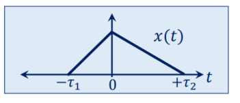
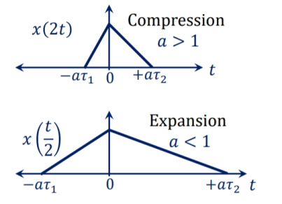
Figure 31. Time Scaling

The resulting signal x(2t) is shown in fig(b). Let x(t) be an audio signal. If x(t) were recorded on a magnetic tape then x(2t) is the signal played back twice the recording speed.

Now consider another signal y(t) = x(at) with a=1/2. Figure ( c ) shows x(1/2) which is expanded in time by factor 2.

In discrete- time signal

y(n) = x(2n)

Let x(n) be a sequence as shown in figure. Then we plot time scaled signal y(n) by substituting different values of n.

For n =-1

y(-1) = x(-2) =2

…..

y(0) = x(0) =4

y(1) = x(2) =2

y(2) = x(4) = 0

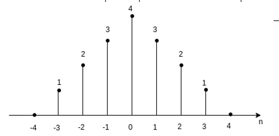
Figure 32. Time scaling in discrete

Signal addition:

The sum of two continuous-time signals can be obtained by adding their values at every instant. Similarly, the subtractions of two continuous-time signals can be obtained by subtracting their values at every instant.

Figure 33. Signal addition

Let us consider the addition and subtraction of two signals x1(t) and x2(t) as shown in Figures (a) and (b).

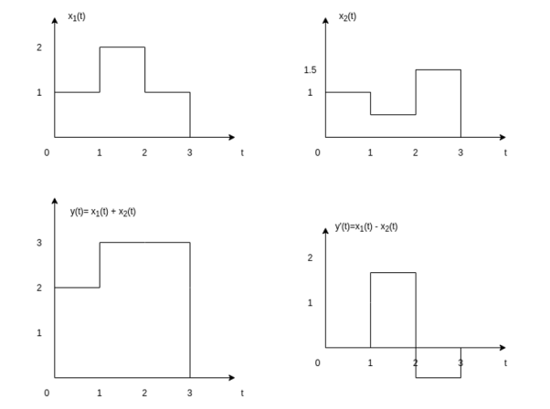
Figure 34. Addition and Subtraction of signal

The addition of signals of two signals x1(t) and x2(t) can be obtained by considering each time interval separately as follows:

x1(t) = 1    for 0 t 1  and

x2(t) =1     for 0 t 1  

Hence x1(t) + x2(t) = 2  for 0 t 1  

x1(t) = 2    for 1 t 2  and

x2(t) =0.5     for 1 t 2

Hence x1(t) + x2(t) = 2.5  for 1 t 2

x1(t) = 1    for 2 t 3  and

x2(t) =1.5     for 2 t 3

Hence x1(t) + x2(t) = 2.5  for 2 t 3

The sketch for y(t) = x1(t) + x2(t) as shown in fig ( c )

In the same way the subtraction of x2(t) from x1(t) can be obtained. By inspection we can find

y’(t) = x1(t) – x2(t)  = 0   for 0 t 1

= 1.5  for 1

= -0.5 for 2 t 3

For discrete-time signals, the sum of two sequences can be obtained by adding the sequence values at the same index n for which the sequences are defined.

Figure 35. Addition of signal in discrete time

If x1(n) = {1, 3, 2, 1}   and

x2(n) = {1, -2, 3, 2}

Then

x1(n) + x2(n) = { 1+1, 3-2, 2+3, 1+2}= {2, 1, 5, 3}

x1(n) – x2(n) = { 1-1, 3-(-2), 2-3, 1-2} = { 0, 5, -1, -1}

Signal Subtraction

The subtraction of two signals is nothing but a subtraction of their corresponding amplitudes.

Consider the following example:

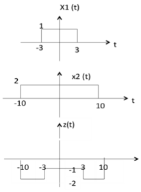
Figure 36. Subtraction of signal in discrete

As seen from the diagram above,

-10 < t < -3 amplitude of z (t) = x1(t) - x2(t) = 0 - 2 = -2

-3 < t < 3 amplitude of z (t) = x1(t) - x2(t) = 1 - 2 = -1

3 < t < 10 amplitude of z (t) = x1(t) + x2(t) = 0 - 2 = -2

Signal multiplication   

The multiplication of two signals can be obtained by multiplying their values at every instant.

The multiplication process is illustrated in the figure.

In the interval 0 t 1

x1(t) = t; x2(t) = 1. Therefore y(t) = x1(t) x2(t)

Therefore y(t) = x1(t) x2(t)=t

In in the interval  1 t 2

x1(t) =1; x2(t) = 0.5. Therefore y(t) = 0.5

In in the interval  2 t 3

x1(t) =0.5; x2(t) = 1.5. Therefore y(t) = 0.75

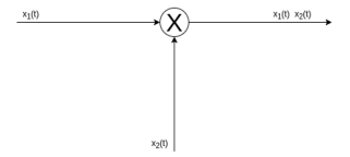
Figure 37. Signal multiplication

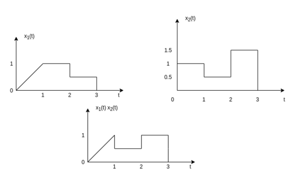
Figure 38. Multiplication of x1 and x2

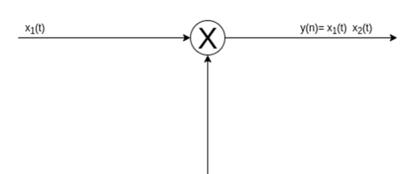
Figure 39. Multiplication of signal in discrete

If x1(n) = { 1, 2, -2, 3} and x2(n) = {1, 0.5, 0.5, 1} then

y(n) = x1(n) . x2(n) ={ 1.1, 2.(0.5), -2(0.5), 3.1}

={1, 1, -1, 3}

Problem:

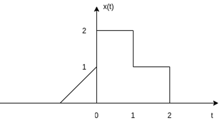
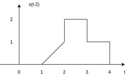
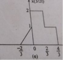
For the signal x(t) as shown in figure find :

(i)                x(t-2)

(ii)              x(2t +3)

(iii)           x(3/2t)

x(t-2)

This signal can be obtained by delaying the signal by 2 units of time.

x(2t+3)

This signal can be obtained first shifting the sequence x(t) left by 3 units of time as shown in fig and then by applying time scaling by factor 2. The resultant signal is shown in the figure.

x(3/2t)

The signal x(3/2t) can be obtained by compressing the signal x(t) by 2/3 times.

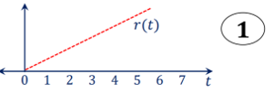
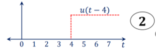
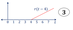
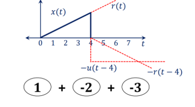
Express the following:

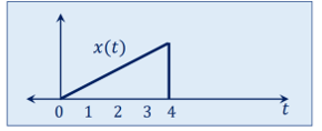
x(t) = r(t) – [ u(t-4) + r(t-4)]

Communication, Control system, and signal processing examples

Control System

•         Industrial control and automation (Control the velocity or position of an object)

•         Examples: Controlling the position of a valve or shaft of a motor

•         Important Tools:

The time-domain solution of differential equations

The transfer function (Laplace Transform)

Stability

Communication

•         Transmission of information (signal) over a channel

•         The channel may be free space, coaxial cable, fiber optic cable

•         A key component of transmission: Modulation (Analog and Digital Communication)

•         Signal processing

•         Signal processing=Application of algorithms to modify signals in a way to make them more useful.

•         Goals:

•         Efficient and reliable transmission, storage, and display of information

•         Information extraction and enhancement

•         Examples:

•         Speech and audio processing

•         Multimedia processing (image and video)

•         Underwater acoustic

•         Biological signal analysis

•         =Application of algorithms to modify signals in a way to make them more useful.

•         Goals:

•         Efficient and reliable transmission, storage, and display of information

•         Information extraction and enhancement

•         Examples:

•         Speech and audio processing

•         Multimedia processing (image and video)

•         Underwater acoustic

•         Biological signal analysis

Key Takeaways

1. The operation of signals in continuous time
2. The operations of signals in discrete time
3. Signals its role in communication and processing

1.4 Classification of signals:

Deterministic

A signal is said to be deterministic if there is no uncertainty with respect to its value at any instant of time or the signals which can be defined exactly by a mathematical formula are known as deterministic signals.

Figure 40. Deterministic signal

Random

A signal is said to be non-deterministic if there is uncertainty with respect to its value at some instant in time. Non-deterministic signals are random in nature hence they are called random signals. Random signals cannot be described by a mathematical equation. They are modeled in probabilistic terms.

Figure 41. Random signal

Periodic

A signal is said to be periodic if it satisfies the condition x(t) = x(t + T) or x(n) = x(n + N).

Where

T = fundamental time period,

1/T = f = fundamental frequency.

Figure 42. Random signal

The above signal will repeat for every time interval T0 hence it is periodic with period T0.

Non-periodic

Non-periodic signals (also known as aperiodic signals), unlike periodic signals, do not have just one particular frequency. Instead, they are spread out over a continuous range of frequencies. For example, a speech signal

Energy

A signal is said to be an energy signal when it has finite energy

Energy E = 2(t) dt

Power:

A signal is said to be a power signal when it has finite power.

Power P = lim T-> ∞ 1/2T   2 (t) dt

Causal and Non-casual

A system is said to be causal if its output depends upon present and past inputs, and does not depend upon future input. For a non-causal system, the output depends upon future inputs also.

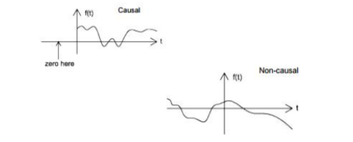
Figure 43. Casual and Non-casual system

Even and odd signal.

A signal is said to be even when it satisfies the condition x(t) = x(-t)

Example 1: t2, t4… cost, etc.

Let x(t) = t2

x(-t) = (-t)2 = t2 = x(t)

∴,∴, t2 is even function

Example 2: As shown in the following diagram, rectangle function x(t) = x(-t) so it is also even function.

Figure 44. Even signal

A signal is said to be odd when it satisfies the condition x(t) = -x(-t)

Example: t, t3 ... And sin t

Let x(t) = sin t

x(-t) = sin(-t) = -sin t = -x(t)

∴,∴, sin t is odd function.

Any function ƒ(t) can be expressed as the sum of its even function ƒe(t) and odd function ƒo(t).

ƒ(t ) = ƒe(t ) + ƒ0(t )

Where

ƒe(t ) = ½[ƒ(t ) +ƒ(-t )]

Key Takeaways:

1. Signals classifications
2. Its importance

1.5 Introduction

A system is defined as a physical device that generates a response or output signal for the given input signal.

The relation between input and output is denoted as

y(t) operation on x(t)

Mathematically

y(t )= T[x(t)]

Where input x(t) is transformed to y(t).  

Figure 45. System

      Classification of Systems

Lumped Parameter and Distributed Parameter

In the lumped parameter system each and every component is lumped at one point in space. These systems are described by ordinary differential equations.

In distributed parameter systems the signals are functions of space as well as time. These systems are described by partial differential equations.

Static and Dynamic systems

A system is static or memoryless if its output at any instant of time depends on the input at that instant of time but not on the past or future values of input. Otherwise, the system is dynamic or with memory.

Examples

y(t) = x 2 (t)           in continuous time     Static or memory less

y(n) = n x(n)          in discrete time        system

Find whether the following systems are dynamic or not:

a)     y(t) = x(t-2)

Here, the output depends on the past value of input therefore the system is dynamic

b)    y(n) = x(n+2)

The output depends on the future value of the input. Therefore, the system is dynamic.

c)     y(t) = x2(t)

The output depends on the present input. Therefore, the system is static.  

Casual and Non-casual systems

A causal system is one for which the output at any time depends on the present and past inputs but not future inputs These systems are known as non- anticipative systems.

A non-casual system is one whose output depends on future values.

Examples of casual system:

y(t) = x(t) + x(t-1)

y(n) = n x(n) + x(n-3)

Examples of non-casual system

y(t) = x(t+3) + x 2 (t)

y(n) = x(2n)

For example

y(t) = 2 x(t) + 3 x(t-3)

Let t=1 therefore y (1) = 2 x(1) + 3 x(-2)

The system output only depends upon present and past inputs. Hence, the system is causal.

y(t) = 2 x(t) + 3 x(t – 3) + 6 x( t+3)

Let t=1 the system output is

y(1) = 2x(1) + 3 x(-2) + 6 x( 4)

Here the output depends future input. Hence non –casual.

 Linear and Non-linear systems

The superposition principle states that the response to a weighted sum of input signals be equal to the weighted sum of the outputs corresponding to each of the individual input signals. A system that satisfies the superposition principle is said to be the linear system.

T [a1 x1(t) + a2 x2(t)] = a1 T[x1(t)] + a2 T[x2(t)]

∴, T [a1 x1(t) + a2 x2(t)] = a1 y1(t) + a2 y2(t)

Similarly, for discrete –time linear system

T [ax1(n) + bx2(n)] = a T[x1(n) + bTx2(n)]

Example:

Check whether the systems are linear or not.

a) dy/dt + 3t y(t) = t2 x(t)

b) y(t) =

c) y(n) = Ax(n) + B

Solution:

a)     dy/dt + 3t y(t) = t2 x(t)

For input x1(t) the output is y1(t)

Dy1(t)/dt + 3t y1(t) = t2 x1(t) --------- (1)

Similarly, for x2(t) output is y2(t)

Dy2(t)/dt + 3t y2(t) = t2 x2(t) ---------- (2)

Multiply (1) with a and (2) with b

a dy1(t) /dt + 3at y1(t) + b dy2(t)/dt + 3by2(t) = at2 x1(t) + bt2 x2(t)

d/dt[ay1(t) +by2(t)] + 3t[ay1(t) + by2(t)] = t2[ax1(t) + bx2(t)]

The system is linear because weighted sum of inputs produces the corresponding weighted sum of outputs.

b)    y(t) =

For x1 input output is y1(t)

y1(t) =

y2((t)

Linear combination of both yields

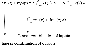
Therefore, system is linear.

c)     y(n) = Ax(n) + B

For input x1(n) the corresponding output is y1(n)

y1(n) = T[x1(n)] = Ax1(n) + B; y2(n) = Tx2(n)] = A x2(n) + B

Ay1(n) + by2(n) = a[Ax1(n) + B] + b[Ax2(n) +B]

The output will be y3(n) = A[x1(n) + x2(n)] +B

y3(n) ≠ ay1(n) + by2(n)

Therefore, system is non-linear.

d)    y(t) = e x(t)

y1(t) = e x1(t)

y2(t) = e x2(t)

y3(t) = T[ax1(t) + b x2(t)] = e[ax1(t)+bx2(t)]

Ay1(t) + by2(t) = a ex1(t) + b ex2(t)

y3(t) ≠ ay1(t) + b y2(t)

Hence, system is not linear.

Time-Variant and Time-invariant systems

A system is said to be time-variant if its input-output characteristics do not change with time.

Suppose we apply a signal(t) to a system to a system and obtain an output y(t) as shown in the figure.

If we delay by T seconds then for a time-invariant system the output will be delayed by T seconds.

Example

Determine whether the following systems are time variant or time invariant.

a)     y(t) = x(t) cos 50πt

b)    y(t) = e x(t)

c)     y(t) = x(t2)

d)    y(n) = x2(n-1)

a)     y(t) = x(t) cos 50πt

If the input is delayed by T sec then output

y(t, T) = T[x(t-T)] = x(t-T) cos (50πt)

If the output is delayed by T sec then

y(t-T) = x(t-T) cos 50 π(t –T)

y(t, T) ≠ y(t – T)

Hence the system is time-variant.

b)    y(t) = ex(t)

The output for delayed input is

y(t, T) = e x(t-T)

The delayed output is

y(t-T) = ex(t-T)

y (t, T) = y(t-T)

Hence, system is time-invariant.

c)y(t) = x(t2)

The output for delayed input is

y(t, T) = x (t2 –T)

The delayed output is

y(t-T) = x(t-T)2

y(t, T) ≠ y(t – T)

Hence the system is a time variant

d)y(n) = x2 (n-1)

The output for delayed input is

y(n-k) = x2(n-1-k)

The delayed output is

y(n-k) = x2 (n-1-k)

y(n, k) = y(n-k)

System is time invariant.

Stable and unstable systems.

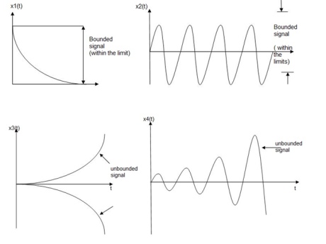
Figure 46. Stable and unstable systems

An input signal x(t) is said to be bounded if it satisfies the condition |x(t) |≤Mx < ∞ for all t.

Similarly, the output signal is bounded if it satisfies the condition |y(t)| ≤My < ∞

The example for bounded and unbounded signals is as shown in the figure.

Note: For a bounded signal, the amplitude is finite.

Example 1: y (t) = x2(t)

Let the input is u(t) that is unit step then output y(t) = u2(t) = u(t) = bounded output.

Hence, the system is stable.

Example 2: y (t) = ∫x(t)dt∫x(t)dt

Let the input be u (t) then

Output y(t) = ∫u(t)dt   but  ∫ u(t)dt = ramp signal

It is unbounded because the amplitude of ramp is not finite and tends to become infinite when t →infinite

Hence, the system is unstable.

Invertible and non-invertible systems

A system is said to invertible if the input of the system appears at the output.

Figure 47. Invertible and Non-invertible system

Y(S) = X(S) H1(S) H2(S)

= X(S) H1(S) · 1(H1(S))/ (H1(S))   Since H2(S) = 1/( H1(S) )

∴, Y(S) = X(S)

→ y(t) = x(t)

Hence, the system is invertible.

If y(t) ≠ x(t), then the system is said to be non-invertible.

To test whether the system is invertible or not:

• If the system produces zero output for any input the system is non-invertible.
• If the system gives the same output for different inputs the system is non-invertible.

Problem:

Determine if the following systems are invertible or not.

a)     y(t) = cos[x(t)]

For input signals separated by 2 π the system gives the gives the same output . Hence system is non-invertible.

b)    y(t) = x(t-3)

Invertible: The inverse system is x(t+3)

c)     y(t) = dx(t)/dt

If x(t) is constant then the output is zero. Therefore, system is non-invertible.

d)    y(n) = x(n)x(n-2)

For input  and   the output is zero. Hence the system is non-invertible.

Check whether the following systems are

     Static or dynamic

     Linear or Non-linear

     Causal or non-casual

     Time-Invariant or time-variant

a)     y(t) d2y(t) /dt2 + 3t dy(t)/dt + y(t) = x(t)

• Since it is a differential equation the system is dynamic.
• The input x1(t) and output y1(t) can be described by

y1(t) d2 y1(t)/dt2 + 3t dy1(t)/dt + y1(t) = x1(t)

Similarly, y2(t) d2y2(t)/dt2 + 3t dy2(t)/dt + y2(t) =x2(t)

a y1(t) d2y1(t)/dt2 + 3at dy1(t)/dt + a y1(t) + b y2(t) d2y1(t)/dt2 + 3bt dy1(t)/dt +by2(t) = ax1(t) + b x2(t)

Ay1 d2 y1(t)/dt2 + by2(t) d2 y(t)/dt2 + 3t d/dt[ay1(t) + b2 y2(t)] + ay1(t) + b y2(t) = ax1(t) + bx2(t)

Since the differentiation ay1(t) d2 y1(t)/dt2 + by2(t) d2 y2(t)/dt2 is not a function of the weighted sum of outputs, superposition principle is not satisfied hence the system is non-linear.

• The output depends on the present input only hence the system is causal.
• The co-efficient of the differential equations is a function of time. Hence the system is time-variant.

y(n) = x(n) x(n-1)

The output depends on the past values of input. Hence it requires memory therefore the system is dynamic.

The output y1(n) for input x1(n) is

y1(n) = x1(n) x1(n-1)

y2(n) = x2(n) x2(n-1)

y3(n) = ax1(n) + b x2(n) [ax1(n-1) + b x2(n-1)]

a y1(n) + by2(n) = a x1(n) x1(n-1) + bx2(n) x2(n-1)

Since y3(n) ≠ ay1(n) + b y2(n)

Hence the system is non-linear.

The output depends on the present and past values of input. Hence the system is casual.

y(n) = x(n) x(n-1)

y (n, k) = x(n-k) x(n-1-k)

y(n-k) = x(n-k) x(n-1-k)

Since y(n, k) = y(n-k) the system is time-invariant.

b)    y (n) = cos[x(n)]

The output depends on the input at that instant. Therefore, system is static.

For input x1(n)

y1(n) = cos[x1(n)]

For input x2(n)

y2(n) = cos[x2(n)]

y3(n) = cos[ax1(n)+ b x2(n)]

a y1(n) + b y2(n) = a cos [x1(n)] + b cos[x2(n)]

Hence the system is non-linear.

The output depends on the present input hence the system is casual.

y(n) = cos[x(n)]

y(n, k) = cos[x(n-k)]

y(n-k) = cos[x(n-k)]

y(n, k) = y(n-k)

Hence system is time –invariant.

For the given system check whether the system is linear, time-invariant, casual memoryless, or stable.

y(t) = x(t-2) + x(2-t)

• The system is not memoryless since the output depends on the past and future values of input.
• The system is non-casual since output depends on the future values of input.

y (t, = x1(t-2-)+x1(2-t-)

y(t-) = x(t-2-) + x2(2-t+)

y (t,  ≠ y (t-

System is time variant.

y1(t) = x1(t-2) + x1(2-t)

y2(t) = x2(t-2) + x2(2-t)

a1y1(t) + a2 y2(t) = a1 x1(t-2)+ a1x1(2-t) + a2x2(t-2)+a2x2(2-t)

= a1x1(t-2) + ax2(t-2) +a1x1(2-t)+a2 x2(2-t)

= System is linear.

For bounded input, the output is also bounded. Hence the system is stable.

Key Take-Aways

1. System definition
2. Classification of system

References:

     Signals and Systems by Simon Haykin

     Signals and Systems by Ganesh Rao

     Signals and Systems by P. Ramesh Babu

     Signals and Systems by Chitode