Unit 2

Time Domain Representation of LTI systems

2.1 Input Output relation

The input-output relationship of linear time-invariant (LTI) systems. If His an LTI system with impulse response h(t), then the output of the system for any arbitrary input is given by convolution integral,

x(t-) d , t R

The same idea can be applied to a discrete-time system with impulse response h[n]. The output, in this case, is given by the convolution sum,

y[n] = x[n-k], n Z

Figure1. Input-Output relation of LTI system

Key take ways:

1. Concept of convolution integral and convolution sum
2. The input and output relation of the LTI system

2.2 Definition of the impulse response

If the input to the system is unit impulse response, then the output of the system is known as the impulse response of the system denoted by h(n). That is

h(n) = T [ δ(n)]…………………………………………………………..(1)

The arbitrary sequence x(n) can be represented as a weighted sum of discrete impulses given by

x(n) =  δ(n-k) --------------------------------------------(2)

Then the output

y(n) = T [  δ(n-k)] -----------------------------------------------------(3)

Key Takeaways:

1. Definition of the impulse response
2. Derivation for impulse response

2.3 Convolution Sum:

Using the linear property of the system the interchange operator T with the summation k to obtain

y(n) = [ T δ(n-k)] ----------------------------------------------(4)

The response to the shifted impulses is represented as h(n,k)

h(n,k) = T[ δ(n-k)]

Now

y(n) =  h(n,k)  -----------------------------------------------------------(5)

For time-invariant system

h(n,k) =h(n-k) ----------------------------------------------------------------------(6)

Substituting (6) in (5) we get

y(n) =  h(n-k)  ------------------------------------------------------------------(7)

Thus, the output of the LTI system is given by the weighted sum of time-shifted responses.

The sum in eq(7) is termed as convolution sum which is given by

y(n) = x(n) * h(n)  -----------------------------------------------------------------------------(8)

* denotes convolution operation.

Key Takeaways

1. Convolution sum
2. Derivation of convolution sum

Problem:

The impulse response h[n] of a discrete-time LTI system. Determine and sketch the output y[n] of this system to the input x[n]

h[n] = δ[n] + δ[n-1] + δ[n-2]+ δ[n-3]+ δ[n-4]+ δ[n-5]

x[n] = δ[n-2] - δ[n-4]

x[n] * h[n] = x[n] * { δ[n] + δ[n-1] + δ[n-2]+ δ[n-3]+ δ[n-4]+ δ[n-5]}

= x[n] + x[n-1] + x[n-2]+ x[n-3]+ x[n-4]+ x[n-5]

y[n] = δ[n-2]- δ[n-4]+ δ[n-3]- δ[n-5] + δ[n-4]- δ[n-6]+ δ[n-5]- δ[n-7] - δ[n-6]+ δ[n-8]- δ[n-7]+ δ[n-9]}

= δ[n-2]+ δ[n-3]-2 δ[n-6]-2 δ[n-7] + δ[n-8]+ δ[n-9]

y[n] = {0,0,1,1,0,0,-2,-2,1,1}

2.4 Convolution Integral

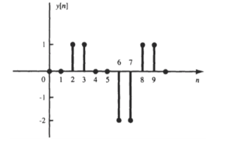
Consider an LTI system that is initially related at t=0. If the input of the system is an impulse, then the output of the system is denoted by h(t) is called the impulse response of the system.

We can denote

h(t) = T [ δ(t)]

We know that any arbitrary signal x(t) can be represented as

x(t) = ( t-d      ------------------------------------------------------(1)

The system output is given by

y(t) = T[x(t)]  --------------------------------------------------------------------------------(2)

Substituting (1) in (2)

y(t) = T [ ( t-d   --------------------------------------------------------(3)

For linear system

y(t) = [ T[ ( t-d --------------------------------------------(4)

If the response of the system due to impulse δ(t) is h(t) then the response of the system due to delayed impulse is

h(t, = T [ δ(t-T)] --------------------------------------------------------------(5)

Substituting (5) in (4) we get

y(t) = [ h(t,τ) dτ -------------------------------------------------------(6)

For a time-invariant system the output due to the delayed input by T is equal to delayed output by T, That is

h(t,τ) = h(t-τ) ---------------------------------------------------------------(7)

Substituting (7) in (6) we get

y(t) =   h(t-τ) dτ  -----------------------------------------------------------(8)

This is called convolution Integral. The convolution of two signal x(t) and h(t) can be represented as

y(t) = x(t) * h(t)

Computation of convolution integral using the graphical method

The procedure is as follows:

1. For the given signals x(t) and h(t) graph the signals x(τ) and h(τ) as a function of independent variable τ.
2. Obtain the signal h(t-τ) by folding h(τ) about τ=0 and then time-shifting by time t.
3. Graph both signals x(τ) and h(t-τ) on the same τ-axis beginning with very large negative time shift t.
4. Multiply the two signals x(τ) h(t-τ) and integrate over the overlapping interval of two signals to obtain y(t)
5. Increase the time shift and take the new interval whenever the function of either x(τ) and h(t-τ) changes. The value of t at which the change occurs defines the end of the current interval and the beginning of a new interval. Calculate y(t) using step 4.
6. Repeat steps 5 and 4 for all intervals.

Unit step to rectangular:

Find the convolution of x(t) and h(t)

x(t) =1                  0

= 0                  otherwise

Fig 2. x(t) and h(t)

Figure 3: x(τ) and h(t-τ)

As shown in Figure the signals x(τ) and h(t-τ) does not overlap for t<0. Therefore the product x(τ) h(t-τ) is zero.

That is,

y(t) = h(t-τ) =0      for t<0

Now the shift the signal h(t-τ) right until the right edge of the signal h(t-τ) intersects the left edge of x(τ).

In the interval 0

y(t) = = t

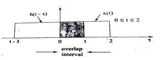
Figure 4. Product of x(t) and h(t-τ)

In the interval 2

y(t) = = 2

In the interval 3

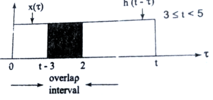
Figure 5. Product of h(t-τ) x(τ)

y(t) = = 2 – (t-3)

= 5-t.

For t

Figure6. Product of x(τ) h(t-τ) for t 5

The signals x(τ) and h(t-τ) do not overlap. Therefore y(t)=0.

y(t) = 0  for t<0

= t   for 1

= 2   for 2

= 5-t  for 3

=0    for t 5.

The sketch y(t) is as shown in figure

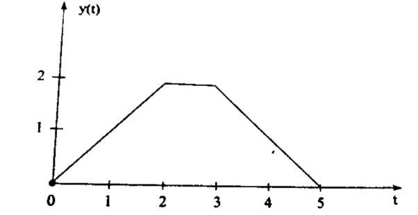
Figure 7. The output waveform

Unit Step to Exponential

Given:

x(t) = e -2 u(t)                      h(t) = u(t+2)

Figure 8. x(t) and h(t)

Figure 9. Product exponential signal and unit step signal

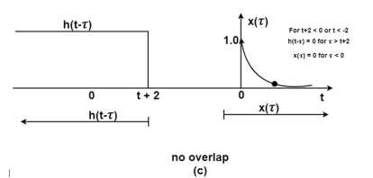
Figure10. Product of exponential signal and delayed unit step signal

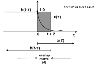
Figure 11. The output waveform

Figure (a) shows x(t) and h(t) . Fig (b) shows x(τ) and h(-τ) as functions of τ. The function h(-τ) can be obtained by folding the signal h(τ) about τ=0.

Figure (c ) shows that signal h(t-τ) is sketched for t<-2 by shifting h(τ) to left. For t<-2 x(τ) and h(t-τ) does not overlap and the product x(τ) h(t-τ) =0 that is

y(t) =0 for t<-2

Now increase the time shift until the signal h(t-τ) intersects x(τ). Figure (d) shows the situation for t>-2.

Here x(τ) =0  for τ <0 and h(t-τ) does not overlap and the product x(τ) h(t-τ) =0 that is

y(t)=0   for t<-2

Now increase the time shift t until the signal h(t-τ) intersects x(τ).

Figure (d) shows the situation for t>-2. Here x(τ) and h(t-τ) overlapped. But x(τ) =0 for τ<0 and h(t-τ) = 0 for τ > t+2. Therefore, the integration interval is from τ=0 to τ=t+2

y(t) = h(t-τ) dτ

= = -2τ dτ

= -1/2 e -2 τ  | 0 t+2

= -1/2 [ e -2 (t+2) -1]

= 1 – e -2(t+2)  /2

y(t) = 0     for t<-2

= 1 – e-2(t+2)/2                 for t -2

Exponential to exponential

x(t) = e -|t|

h(t) = e -2(t+1) u(t+1)

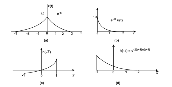
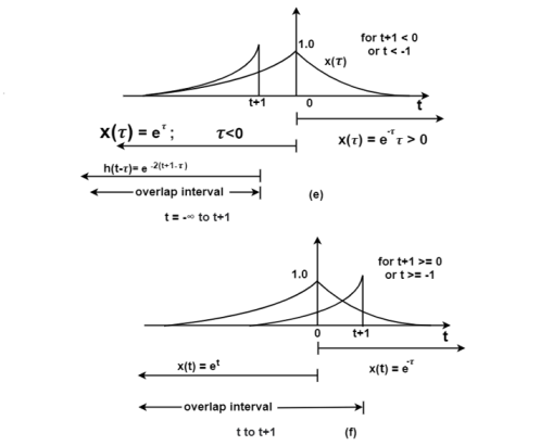
Figure 12. Steps for exponential to exponential convolution

Fig (a) shows the signal x(t). In fig(b) the signal e -2t u(t) is sketched from which can be obtained from the signal h(t) = e -2(t+1) u(t+1)

Fig ( c ) shows the signal h(-τ) which can be obtained by folding the signal h(τ) about t=0.

In fig (e ) the signals x(τ) and h(t-τ) are drawn on the same axis.

For (t+1) <0 or t<-1 the signals x(τ) and h(t-τ) overlap over the interval - τt+1.

During this interval the signal x(τ) = e τ and h(t-τ) = e -2 (t+1-τ). Therefore, for

t<-1

y(t) = τ e -2(t+1-τ) dτ

= e -2t -2 3 τ  dτ

= e -2(t+1) /3 e 3 τ  | - 0  + e -2 (t+1) e τ | 0 t+1

= e -2(t+1) /3 [1] + e –2(t+1)  [ e t+1 -1 ]

= e -2(t+1) /3 + e –(t+1) – e -2 (t+1)

= e –(t+1) – 2/3 e -2(t+1)

y (t) = 1/3 e t+1     for t<-1

= e –(t+1) – 2/3 e -2(t+1)    for t -1

Rectangular to rectangular

Find the response of the system y(t) of an LTI system whose x(t) and h(t) are as shown in the figure.

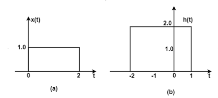
Fig 13. x(t) and h(t) signals

The figure shows the signal x(τ) and h(-τ). In the figure, the signals x(τ) and h(t-τ) do not overlap. Therefore, the product x(τ) h(t-τ) is equal to zero. For t<-2 the signals x(τ) and h(t-τ) does not overlap. Therefore, the product x(τ) h(t-τ) is equal to zero.

Hence

y(t) = h(t-τ) dτ

= 0 for t<-2

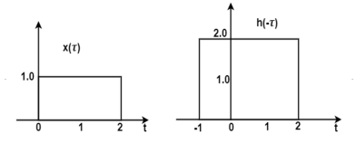
Fig 14. Convolution of x(t) and h(-τ)

Now increase the value of t and shift the signal h(t-τ) as shown in figure. Here the overlap interval is τ = 0 to t+2 . In this interval x(τ) = 1.0 ; h(t-τ) = 2.0

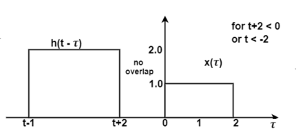
Figure 15. Convolution of x(τ) h(t-τ)

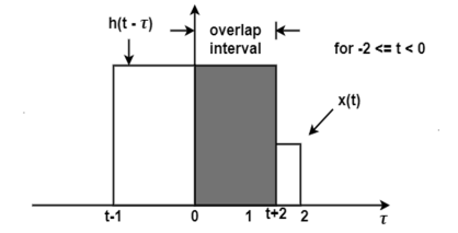
Figure 16. Output of the convolution x(t) and h(t)

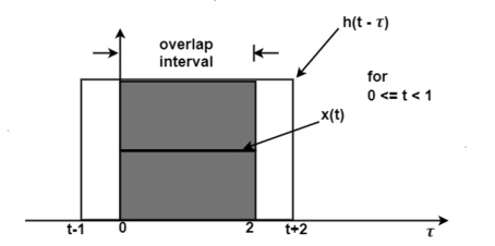
Figure 17. Output for t<1

Therefore,

y(t) =   d τ

= 2τ | 0 t+2 = 2(t+2) = 2t + 4

This value holds for -2

In the interval 0 1 the overlap interval is constant that is from τ=0 to τ=2

Therefore

y(t) =   d τ =2 τ | 0 2 =4

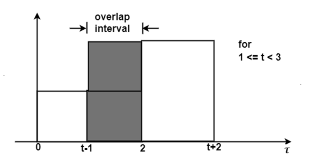
Figure 18. Output waveform for t<3

If we shift h(t-τ) further the resultant diagram is shown in fig 4.29. Here the overlap interval is from τ = t-1 to τ=2. Therefore, for the interval 1

y(t) = dτ

= 2τ | 2 t-1

= 2[ 2 – (t-1)]

= 6 – 2t

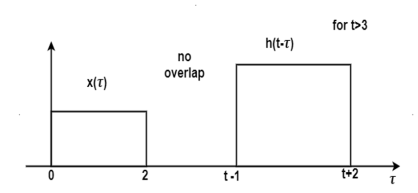
Figure 19. Output waveform for t>3

For t>3 the signals do not overlap. Therefore

y(t) = 0    for t>3

y(t) = 0    for t -2

= 2t + 4   for -2 <0

= 4        for 0 t <1

= 6 -2t      for 1 <3

=0         for t

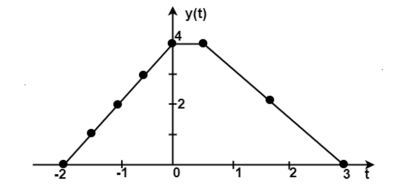
Figure 20. Final output waveform

Unit step to unit step

x(t) = u(t+1)              h(t) = u(t-2)

The signals x(t) and h(t) are shown in figure.

Figure 20. Unit step signal x(t)

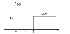
Figure 21. Unit step signal

The figure below the signals x(τ) and h(t-τ) on the same axis. The signal h(t-τ) is obtained by folding the signal h(τ) about τ=0 and then left shifting h(-τ).

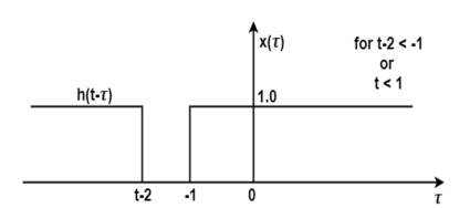
Figure 22. Convolution of x(τ) and folding signal h(t-τ)

For t<1 the overlap area of x(τ) and h(t-τ) is zero. Therefore y(t) =0. Now shift the signal h(t-τ) right as shown in the figure.

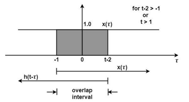
Figure 23. Convolution for t>1

Here the signal x(τ) and h(t-τ) do overlap over the interval -1 < t-2 . Therefore

y(t) = h(t-τ) d τ

= τ | -1 -2  = (t-2) – (-1) = t-1

= y(t) =0 for t<1

= t-1 for t 1

The signal y(t) is sketched as shown in figure.

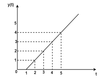
Figure 24. The output waveform

Key Takeaways:

1. Definition of convolution integral and its derivation
2. Procedure for graphical representation
3. Representation for various signals like step, exponential, and so on.

2.5 Computation of convolution sum

For x(n) = {3,2,-1,2,4,1} find the sum of the shifted unit impulses.

Given x(n) = {3,2,-1,2,4,1}

-1,0,1,2,3,4

x(-1) = 3. x(0)=2 , x(1)=-1, x(2) =2, x(3)=4,x(4) =1

x(n) = δ(n-k)

x(-1) δ(n+1) + x(0) δ(n) + x(1) δ(n-1) + x(2) δ(n-2)+ x(3) δ(n-3)+ x(4) δ(n-4)

We get

3 δ(n+1) + 2 δ(n) - δ(n-1) + 2 δ(n-2)+ 4 δ(n-3)+ δ(n-4)

Key take ways

1. Computation of convolution sum

2.6 Properties of Convolution Sum

Commutative Property

The commutative property states that the order in which two sequences are convolved is not important. Mathematically, the commutative property is

x(n) * h(n) = h(n) * x(n)

From a systems point of view, this property states that a system with a unit sample response h(n) and input x(n) behaves in the same way as a system with unit sample response x(n) and an input h(n).

This is illustrated in Fig. (a).

Associative Property

The convolution operator satisfies the associative property, which is

[x(n) * h1(n) } * h2(n) = x(n) * { h1(n) * h2(n)}

From a systems point of view, the associative property states that if two systems with unit sample responses h1(n) and h2(n) are connected in cascade as shown in Fig. (b), an equivalent system is one that has a unit sample response equal to the convolution of h1 (n) and h2(n):

Heq = h1(n) * h2(n)

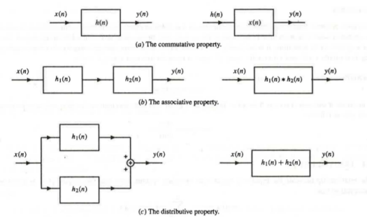
Figure 25. Commutative, Associative, and Distributive Property.

Distributive Property

The distributive property of the convolution operator states that

x(n) * {hl(n) + h2(n)} = x(n) * hJ(n) + x(n) * h2(n)

From a systems point of view, this property asserts that if two systems with unit sample responses h J (n) and h2(n) are connected in parallel, as illustrated in Fig. (c), an equivalent system is one that has a unit sample response equal to the sum of hJ(n) and h2(n):

Heq (n) = h1(n) + h2(n)

Key takeaways:

• Properties of convolution sum
• Its applications

2.7 System Interconnections

Parallel connection:

Consider two LTI systems with impulse responses h1 (t) and h2 (t) connected in parallel, as illustrated in Fig. (a), the output of this connection of systems, y(t), is the sum of the outputs of the two systems:

𝑦 (𝑡 )= 𝑦1 (𝑡) + 𝑦2 (𝑡)

= 𝑥( 𝑡) ∗ ℎ1 (t) + 𝑥 (𝑡) ∗ ℎ2( 𝑡)

y(t) = h1(t-τ) dτ + h2(t-τ) dτ = h1(t-τ) dτ

Where h(t-τ) = h1 (t-τ) = h1(t-τ) + h2(t-τ) is the impulse response of the equivalent system.

Figure 26. Parallel connection

Identical results hold for the discrete-time case:

𝑥(𝑛) ∗ ℎ1 + 𝑥 (𝑛 )∗ ℎ2 = 𝑥 (𝑛) ∗[ ℎ1[𝑛] + ℎ2[𝑛] ]

Cascade Connection

Consider the cascade connection of two LTI systems, as illustrated in Fig. (a). Let z(t) be the output of the first system and therefore the input to the second system in the cascade.

The output is expressed in terms of z(t) as 𝑦 (𝑡) = 𝑧(𝑡) ∗ ℎ2(𝑡)

Substituting for z(t), we get

y(t) = h2(t-τ) dτ

Putting for z(t) we get

y(t) = h1(τ-v) h2(t-τ) dv dτ

= h(t-τ) dv

= h(t) * h(t)

Figure 27. Cascade connection

Interconnection of two LTI systems. (a) Cascade connection of two systems. (b) Equivalent system. (c) Equivalent system: Interchange system order.

Problem:

Consider the interconnection of four LTI systems as shown in figure. The impulse responses of the systems are

h1[n] = u[n]

h2[n] = u[n+2] – u[n]

h3[n] = δ[n-2]

And

h4[n] = α n u[n]

Find the impulse response h[n] of the overall system.

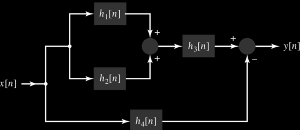
Figure 28. Impulse response h[n]

We first derive the expression for the overall impulse response in the terms of the impulse response of each system.

The parallel com0bination h1[n] and h2[n] . The distributive property implies that the equivalent system h12[n] = h1[n] + h2[n] as shown in figure 1.

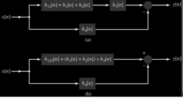
Figure 29. Reduction

This system is in series with h3[n] so the associative property implies that the equivalent system for the upper branch has the impulse response h123[n] = h12[n] * h3[n]

Substituting for h12[n] in this expression we have

h123[n] = (h1[n] + h2[n] * h3[n]) as shown in fig(b) . Last the upper branch is in parallel with the lower branch characterized by h4[n] ; hence application of the distributive property gives the overall system impuse response as h[n] = h123[n] – h4[n]

Substituing for h123[n] in this expression yields

H[n] = ( h1[n] + h2[n] ) * h3[n] – h4[n]

As shown in fig ( c)

Now substitute the specified forms h1[n] and h2[n] to obtain

h12[n] = u[n] + u[n+2] – u[n]

=u[n+2]

Convolving h12[n] with h3[n] gives

h123[n] = u[n+2] * δ[n-2] = u[n]

Finally, we sum h123[n] and -h4[n] to obtain the overall impulse response

h[n] = { 1- α n } u{n}

Figure 30. Output response

Key Takeaways:

• System interconnection and its types
• Reduction of the system using system interconnections

2.8 System properties in terms of the impulse response, step response in terms of the impulse response.

Figure 31. Impulse response and step response

The step response of a discrete-time LTI system is the convolution of the unit step with the impulse response-

s[n]=u[n]*h[n]. -------------------(1)

Commutative property of convolution,

s[n]=h[n]*u[n]. ----------------------------------------(2)

That means s[n] is the response to the input h[n] of a discrete-time LTI system with unit impulse response u[n].

Figure 32. Output response

s[n] = u[n-k]…………………………………(1)

Since u [n- k]< 0 is for n- k< 0, i.e. k> n and 1 for n -k> 0, i.e. k≤ n.

s[n] = ------------------------------------------------(2)

That is the step response of the discrete LTI system is the running sum of its impulse response.

s[n-1] =

s[n] - s[n-1] =  - =

s[n] - s[n-1] = + h[n] - =

h[n] = s[n] – s[n-1]

From here h[n] can be recovered from s[n], the impulse response of the discrete-time LTI system is the first difference of its step response.

For continuous-time system

The unit step response is the running integral of its impulse response.

s(t) = ) dτ

The unit impulse response is the first derivative of the unit step response: -

h(t)= ds(t)/dt = s’(t)

Problem:

Find the step response of the system whose impulse response is given by

(i)                u(t+1) – u(t-1)

s(t) = ) dτ

s(t) = (t+1) – u(t-1) dτ

= τ - τ

= τ |-1 t – τ | 1 t

=(t+1) – (t-1)

=2

(ii)              e -3t u(t) – e-2t u(t)

s(t) = ) dτ

s(t) = -3t dτ + -2t dτ

s(t) = -1/3 [e -3t -1+1/2 [e -2t -1 ]

= -1/3 e -3t +1/3 +1/2 e -2t -1/2

=-1/3 e -3t +1/2 e -2t -1/2

= -1/3 e -3t +1/2 e -2t -1/6  for t 0

x(t) = -1/3 e -3t u(t)+1/2 e -2t u(t)-1/6  u(t)

Key Take-Aways:

1. System properties in terms of the impulse response for unit
2. System properties in terms of the impulse response for unit

References:

     Signals and Systems by Simon Haykin

     Signals and Systems by Ganesh Rao

     Signals and Systems by P. Ramesh Babu

     Signals and Systems by Chitode