Unit 4
Fourier Transform
Aperiodic signals in continuous time are represented by the Fourier transform
An aperiodic signal can be viewed as a periodic signal with an infinite period
As the period becomes infinite, the frequency components form a continuum and the Fourier series becomes an integral
The (CT) Fourier transform (or spectrum) of x(t) is
X(jw) =  e -jwt dt ---------------------------------------(1)
x(t) can be reconstructed from its spectrum using the inverse Fourier transform
x(t) = 1/ 2 π  e jwt dw ------------------------------------------(2)
The above two equations are referred to as Fourier transform pair with the first one being the analysis equation and the second being the synthesis equation.
Notation
X(jw) = F{x(t)}
x(t) = F -1 {X(jw)}
x(t) and X(jw) form a Fourier transform pair denoted by
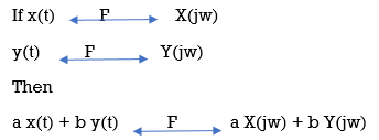
x(t)  F X(jw)
Example :
Rect(t) or π(t) = 1 |t|  ½
½
0 |t| > ½
½ |t| =1/2
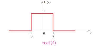
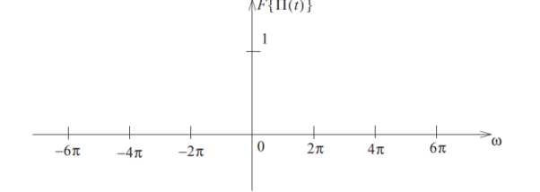
Figure 1. Fourier transform of rect of rect(t)
Key Take-Aways:
- Fourier transform definition
- Fourier transform notation
- f(x) must integrable over a period.
- f(x) must have a finite number of exterma in any given interval, i.e. there must be a finite number of maxima and minima in the interval.
- f(x) must have a finite number of discontinues in any given interval, however, the discontinuity cannot be infinite.
- f(x) must be bounded.
The last three conditions are satisfied if f is a function of bounded variation over a period.
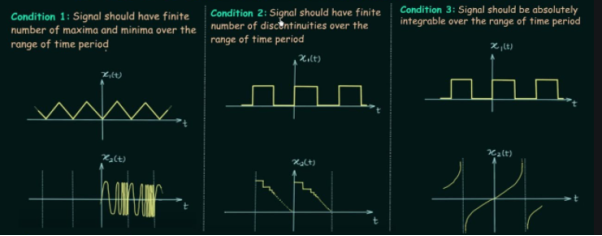
Figure 2. Dirichlet condition
Key Take-Aways:
- Dirichlet condition for Fourier transform
- The three conditions that satisfy Dirichlet condition
H(e jw) = H R ( e jw) + j H I ( e jw) = | H ( e jw) | e j  1 (w)
1 (w)
 1 (w) = angle H(e jw)
Example:
h[n] = - δ[n]
| H (ejw)| = 1 angle H(e jw) = π
In the magnitude or phase representation, a real-valued frequency response does not mean that the system is zero-phase.
Using this representation,
|Y (e jw) | = | H ( ejw)| | X (ejw)|
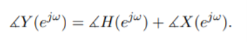
Thus, |H(ejω)| and angle H(ejω) is commonly referred to as the gain and the phase shift of the system, respectively.
In magnitude and phase plots, as ω goes through a zero on the unit circle, the magnitude will go to zero and the phase will flip by π, as shown in the figure below.
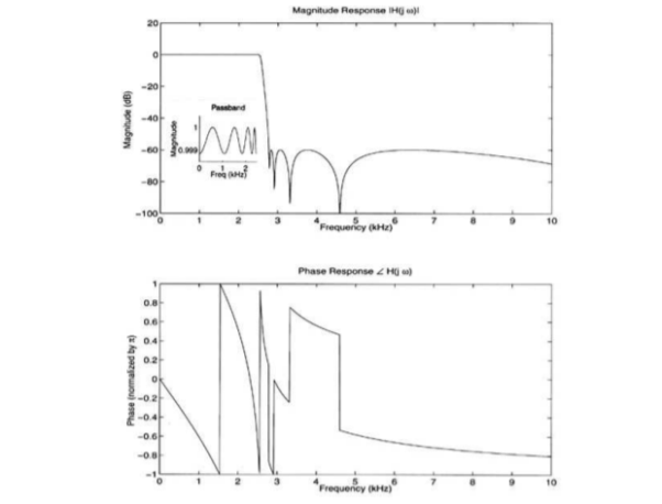
Figure 3. Magnitude and Phase response
Key Take-Aways:
- Magnitude response
- Phase response
Starting from the Fourier series representation for the continuous-time periodic square wave:
x(t) = { 1 |t| < T1
0 T1 < |t| < T/2
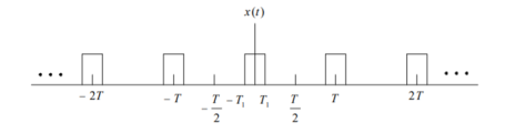
Figure 4. Fourier transform of a standard continuous-time signal
The Fourier coefficients ak for this square wave are
Ak = 2 sin(kwoT1) / kwoT ----------------------------------------------------------------(2)
Alternatively
Tak = 2 sin(wT1)/w | w=kwo
Where 2 sin(wT1)/w represents the envelope of Tak. -----------------------------(3)
When T increases or the fundamental frequency w0 = 2p /T decreases, the envelope is sampled with closer and closer spacing.
As T becomes arbitrarily large, the original periodic square wave approaches a rectangular pulse. · Tak becomes more and more closely spaced samples of the envelope, as T -> ∞ , the Fourier series coefficients approaches the envelope function.
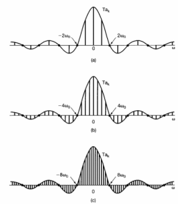
Figure 5. Envelope function
As T->∞ x˜(t) = x(t) for any infinite value of t.
The Fourier series representation of x˜(t) is
x˜(t) =  e j wot ----------------------------------------------------------------------(4)
Ak = 1/T  e j wot dt ----------------------------------------------------------------(5)
Since  = x(t) for |t| < T/2 and also since x(t) =0 outside the interval so we have
Ak = 1/T  e j wot dt = 1/T 1/T
  e j wot dt
Define the envelope X(jw) of T ak as
X(jw) =  e j wt dt -----------------------------------------------(6)
We have for the co-efficient ak
Ak = 1/T X(jkwo)
Then  can be expressed in terms of X(jw) that is
 =
=  X(jkwo)e j kwot -= 1/2π
 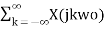 e j kwot wo
As T -> ∞  = x(t) and hence the above equation becomes a representation of x(t).
Besides, w0 -> 0 as T ->∞ , and the right-hand side of Eq. (7) becomes integral.
x(t) = 1/2π  e jwt dw Inverse Fourier Transform
X(jw) =  e -jwt dt Fourier transform
Key Take-Aways :
- Fourier transform for standard continuous-time signal
- Envelope function
(i) Linearity
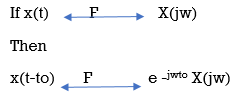
(ii) Time shifting
Find the Fourier transform of the signal as shown in figure
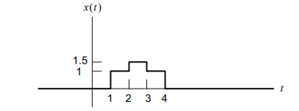
Figure 6. Input signal
This signal can be obtained as a linear combination of
x(t) = ½ x1(t-2.5) + x2(t-2.5)
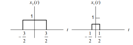
Figure 7. Combination of x1(t) and x2(t)
Where x1(t) and x2(t) are rectangular pulse signals and their Fourier transforms are
X1(jw) = 2 sin (w/2) / w and X2(jw) = 2 sin (3w/2)/w
Using linearity and time shifting properties of Fourier transform yields
X(jw) = e -j5w/2 { sin(w/2) + 2 sin(3w/2) /w}
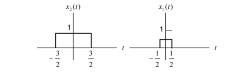
Figure 8. The output waveform
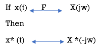
Conjugate Property:
Differentiation and Integration
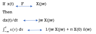
Consider the Fourier transform of the unit step x(t) = u(t).
We know that
Also note that
x(t) =  ) dτ
) dτ
The fourier transform of this function is
X(jw) = 1/jw + π G(0) δ(w) = 1/jw + π δ(w)
Where G(0) =1 .
Find the Fourier transform of the function x(t) as shown in the figure.
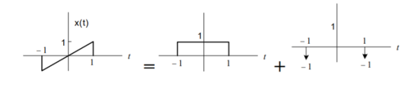
Figure 9. Input signal x(t) and its interpretation
From the above figure, we see that g(t) = d x(t) /dt is a sum of a rectangular pulse and two impulses.
G(jw) = (2 sin w/w) – e jw – e -jw
Using integration property we obtain
X(jw) = G(jw) / jw + π G(0) δ(w) = 2 sin w/ j w 2 – 2 cos w / jw
It can be found that X(jw) is purely imaginary and odd which is consistent with the fact that x(t) is real and odd.
Time and Frequency scaling
Then
x(at) = 1/ |a| X(jw/a)
Parseval’s relation
We have
 x(t)| 2 dt = 1/ 2 π
  X(jw)| 2 dw
Parseval’s relation states that the total energy may be determined either by computing the energy per unit time |x(t)| 2 and integrating over all the time by computing the energy per unit frequency |X(jw)| 2 / 2 π and integrating over all frequencies.
For this reason |X(jw)| is often referred to as the energy-density spectrum.
Convolution properties

Multiplication property

Multiplication of one signal by another can be thought of as one signal to scale or modulate the amplitude of the other consequently the multiplication of two signals is referred to as amplitude modulation.
Key Take-Aways:
- Properties of Fourier transform
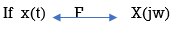
A unit rectangular window function rect(x) is given by
Rect(x) = { 0 |x| >1/2
½ |x| = ½
1 |x| <1/2
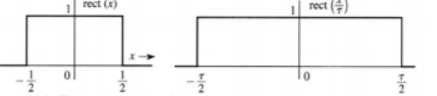
Figure 10. Rectangular window function
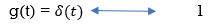
The unit impulse function δ(t) Dirac impulse
δ(t) =0 t 0
0
 dt =1
dt =1
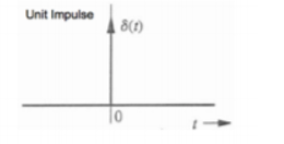
Figure 11. Unit impulse function
Interpolation function
Sinc(x) = sin x/x or sinc(x) = sin πx/πx
The rectangular function often called a “window” because when we multiply it with a signal it lets some signals pass through and blocks the other. We sample a continuous-time signal to obtain a discrete-time signal.
The sinc(x) = sinx/x function
When we evaluate
X(w) =  (t/τ) e -jwt dt
Since rect(t/τ) =1 for -τ/2 <t<τ/2 and 0 otherwise
X(w) =  e -jwt dt
= -1/jw ( e -jw/2 – e jw/2) = 2 sin(wt/2) / w = τ . Sin(wτ/2)/(wτ/2) = τ . Sinc(wτ/2)
Rect(t/τ) -> τ sinc (wτ/2)
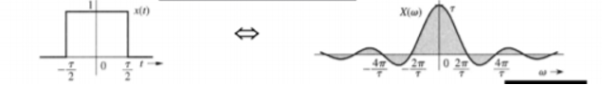
Figure 12. Sinc function
The frequency of the original signal is changed according to the sinc function – a spectral function of a rectangular window. This is done through a process called convolution.
Key Take-Aways:
- The relation between time and frequency domain
- Sinc function
We know that the Fourier transform of the signal assumes the value 1 identically is the Dirac-delta function.
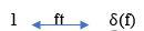
By the property of translation in the frequency domain we get
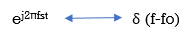
Suppose x(t) is a periodic signal with period T which admits Fourier series representation Then
x(t) =  e j2πkfst
Where
Ck = 1/T  e -j2πkfst dt
Since the Fourier transformation is linear the above result can be used to obtain the Fourier transform of the periodic signal
X(f) =  (Fourier transform of e j2π/TjkT
Therefore
X(f) =  δ(f-k/T)
By putting the inverse Fourier transform equation one can indeed confirm that one obtains the Fourier series representation of x(t)
 e j2πft df =
  k δ(f-k/T) e j2πft df
=  k δ(f-k/T) e j2πft df
=  k e j2π k/f.t
Thus, the Fourier transform of a periodic signal having the Fourier series coefficients is a train of impulses, occurring at multiples of the fundamental frequency, the strength of the impulse at k/T being ck which looks like
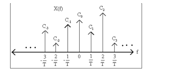
Figure 13. Fourier representation of periodic signals
Key Take-Aways:
- Fourier representation of periodic signals
- Derivation and its spectrum
References
Signals and Systems by Simon Haykin
Signals and Systems by Ganesh Rao
Signals and Systems by P. Ramesh Babu
Signals and Systems by Chitode


