Unit 6 | unit 6 probability and random variables

S&S

Unit 6

Probability and Random Variables

6.1 Experiment, Sample space, Event

In the probabilistic situation that we analyze can be viewed in the context of an experiment. By experiment, we mean any nondeterministic process that has a number of distinct possible outcomes. Thus, an experiment is first characterized by a list of possible outcomes.

A particular performance of the experiment, sometimes referred to as an experimental trial, yields one and only one of the outcomes.

The finest-grained list of outcomes for an experiment is the sample space of the experiment. Examples of sample spaces are:

{heads, tails) in the simple toss of a coin.
[1, 2, 3 .... 1, describing the possible number of fire alarms in a city during a year.
{0 x 10, 0 y 10), describing the possible locations of required on-the-scene social services in a city 10 by 10 miles square.

As these three examples indicate, the number of elements or points in a sample space can be finite, countably infinite, or uncountably infinite. Also, the elements may be something other than numbers (e.g., "heads" or "tails").

Probabilistic analysis requires considerable manipulation in an experiment's sample space. For this, we require knowledge of the algebra of events, where an event is defined to be a collection of points in the sample space. A generic event is given an arbitrary label, such as A, B, or C. Since the entire sample space defines the universe of our concerns, it is called , for the universal event. An event containing no points in the sample space is called o, the empty event (or null set).

Events A1 A2, . . . , AN are said to be collectively exhaustive if they include all points in the universe of events:

A set of events A1, A2,..., AN that are both mutually exclusive and collectively exhaustive contains each point of the sample space U in one and only one of the events Ai

Key Take-Aways:

Definition for experiment
Definition of event
Definition of sample space

6.2 Probability, Conditional Probability, and Statistical Independence

Probability is the measure of the likelihood that an event will occur in a Random Experiment. Probability is quantified as a number between 0 and 1, where, loosely speaking, 0 indicates impossibility and 1 indicates certainty. The higher the probability of an event, the more likely it is that the event will occur.
Example
A simple example is the tossing of a fair (unbiased) coin. Since the coin is fair, the two outcomes (“heads” and “tails”) are both equally probable; the probability of “heads” equals the probability of “tails”; and since no other outcomes are possible, the probability of either “heads” or “tails” is 1/2 which could also be written as 0.5 or 50%.

Conditional probabilities arise naturally in the investigation of experiments where an outcome of a trial affects the outcomes of the subsequent trials.

We try to calculate the probability of the second event (event B) given that the first event (event A) has already happened. If the probability of the event changes when we take the first event into consideration, we can safely say that the probability of event B is dependent of the occurrence of event A.

For example

Drawing a second ace from a deck given we got the first ace
Finding the probability of having a disease given you were tested positive
Finding the probability of liking Harry Potter given we know the person likes fiction

Here there are 2 events:

Event A is the probability of the event we are trying to calculate.
Event B is the condition that we know or the event that has happened.

Hence we write the conditional probability as P ( A/B), the probability of the occurrence of event A given that B has already happened.

P(A/B) = P( A and B) / P(B) = Probability of occurrence of both A and B / Probability of B

Suppose you draw two cards from a deck and you win if you get a jack followed by an ace (without replacement). What is the probability of winning, given we know that you got a jack in the first turn?

Let event A be getting a jack in the first turn

Let event B be getting an ace in the second turn.

We need to find P(B/A)

P(A) = 4/52

P(B) = 4/51 {no replacement}

P(A and B) = 4/52*4/51= 0.006

P(B/A) = P( A and B)/ P(A) = 0.006/0.077 = 0.078

Here we are determining the probabilities when we know some conditions instead of calculating random probabilities

Statistical Independence

Statistical independence is a concept in probability theory. Two events A and B are statistically independent if and only if their joint probability can be factorized into their marginal probabilities, i.e.,

P(A ∩ B) = P(A)P(B).

If two events A and B are statistically independent, then the conditional probability equals the marginal probability:

P(A|B) = P(A) and P(B|A) = P(B).

The concept can be generalized to more than two events. The events A1, …, An are independent if and only if

P(⋂i=1n Ai)=∏i=1 nP(Ai)

Key Take-Aways:

Definition of Probability
Definition of Conditional Probability
Definition of Statistical Dependence

6.3 Baye’s theorem

The Bayes theorem describes the probability of an event based on the prior knowledge of the conditions that might be related to the event.

If we know the conditional probability P(A/B), we can use the Bayes rule to find out the reverse probabilities P(B/A).

How can we do that?

P(A/B) = P ( A B) / P(B)

P(B/A) = P ( A B) / P(A)

P ( A B) = P(A/B) * P(B) = P(B/A) * P(A)

P(B/A) = P(A/B) * P(B)/ P(A)

The above statement is the general representation of the Bayes rule.

Example

Rahul’s favourite breakfast is bagels and his favourite lunch is pizza. The probability of Rahul having bagels for breakfast is 0.6. The probability of him having pizza for lunch is 0.5. The probability of him, having a bagel for breakfast given that he eats a pizza for lunch is 0.7.

To calculate the probability of having a pizza for lunch provided you had a bagel for breakfast would be = 0.7 * 0.5/0.6.

Key Take-Aways :

Baye’s theorem
Representation of Baye’s theorem

6.4 Uniform and Gaussian Probability models

A probability model is a mathematical representation of a random phenomenon. It is defined by its sample space, events within the sample space, and probabilities associated with each event.

The sample space S for a probability model is the set of all possible outcomes.

For example, suppose there are 5 marbles in a bowl.

One is red, one is blue, one is yellow, one is green, and one is purple. If one marble is to be picked at random from the bowl, the sample space possible outcomes S = {red, blue, yellow, green, purple}.

If 3 of the marbles are red and 2 are blue, then the sample space S = {red, blue}, since only two possible color outcomes are possible. If, instead, two marbles are picked from a bowl with 3 red marbles and 2 blue marbles, then the sample space

S = {(2 red), (2 blue), (1 red and 1 blue)}, the set of all possible outcomes.

Uniform Probability Model:

A uniform probability model has outcomes that all have the same chance of occurring.
A uniform probability model has outcomes that are not the same for every trial.
A uniform probability model has outcomes that do not all have the same chance of occurring.

Gaussian Probability Model

In order to generalize the model to incorporate two parameters one for central value and the other for spread or scale of the distribution. These are called mean parameters and standard deviation parameters denoted by μ and A variable with such a distribution is derived by multiplying z by the scale factor and adding to get

x= μ + z .

Key Take-Aways:

Uniform probability model
Gaussian probability model

6.5 Continuous and Discrete random variables

A variable is a quantity whose value changes.

A discrete variable is a variable whose value is obtained by counting.

Examples: number of students present

Number of red marbles in a jar

Number of heads when flipping three coins

Students’ grade level

A continuous variable is a variable whose value is obtained by measuring.

Examples: height of students in class

Weight of students in class

Time it takes to get to school

Distance travelled between classes

A random variable is a variable whose value is a numerical outcome of a random phenomenon.

▪ A random variable is denoted with a capital letter

▪ The probability distribution of a random variable X tells what the possible values of X are and how probabilities are assigned to those values

▪ A random variable can be discrete or continuous

A discrete random variable X has a countable number of possible values.

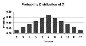
Example: Let X represent the sum of two dice.

Then the probability distribution of X is as follows:

P(X)

To graph the probability distribution of a discrete random variable, construct a probability histogram.

Figure 1. Probability distribution

A continuous random variable X takes all values in a given interval of numbers.

▪ The probability distribution of a continuous random variable is shown by a density curve.

▪ The probability that X is between an interval of numbers is the area under the density curve between the interval endpoints

▪ The probability that a continuous random variable X is exactly equal to a number is zero

Key Take-Aways:

Continuous random variable
Discrete random variable

6.6 Cumulative Distributive function, Probability density function, Properties of CDF and PDF

Cumulative Distributive function

The cumulative distribution function (CDF) of a random variable is another method to describe the distribution of random variables. The advantage of the CDF is that it can be defined for any kind of random variable discrete, continuous, and mixed.

Definition

The cumulative distribution function (CDF) of random variable X is defined as

FX(x)=P(X≤x), for all x∈R.

Note that the subscript X indicates that this is the CDF of the random variable X. Also, note that the CDF is defined for all x∈R. Let us look at an example.

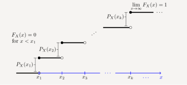
In general, let X be a discrete random variable with range RX={x1,x2,x3,...}, such that x1<x2<x3<... Here, for simplicity, we assume that the range RX is bounded from below, i.e., x1 is the smallest value in RX.

If this is not the case then FX(x) approaches zero as x→−∞ rather than hitting zero. The figure shows the general form of the CDF, FX(x), for such a random variable.

We see that the CDF is in the form of a staircase. In particular, note that the CDF starts at 0; i.e.,FX(−∞)=0. Then, it jumps at each point in the range. In particular, the CDF stays flat between xk and xk+1, so we can write

FX(x)=FX(xk), for xk≤x<xk+1.

The CDF jumps at each xk. In particular, we can write

FX(xk)−FX(xk−ϵ)=PX(xk), For ϵ>0 small enough.

Thus, the CDF is always a non-decreasing function, i.e., if y≥x then FX(y)≥FX(x). Finally, the CDF approaches 1 as x becomes large. We can write

Limx→∞FX(x)=1.

Figure 2. CDF of discrete time variable

Probability density function

In probability theory, a probability density function (PDF), or density of a continuous random variable, is a function that describes the relative likelihood for this random variable to take on a given value.

Probability density function is defined by following formula:

P(a≤X≤b)=

Where −

[a,b][a,b] = Interval in which x lies.
P(a≤X≤b) = probability that some value x lies within this interval.
Dx = b-a

Example

During the day, a clock at random stops once at any time. If x be the time when it stops and the PDF for x is given by:

f(x) = {1/24, 0, for 0 x 24

0 otherwise

Calculate the probability that clock stops between 2 pm and 2:45 pm.

Solution:

We have found the value of the following:

P(14 14.45 )

= dx

= 1/24 (0.45)

= 0.01875

Properties of CDF:

FX (-∞)=0
FX (∞)=1
0≤FX≤1
FX (x1) ≤ FX (x2 ) if x1 < x2 i.e. c.d.f is monotonically increasing function.
P(x1 < X < x2 ) = FX (x2 ) - FX (x1 )
FX (x+ ) = FX (x) . The function is continuous on the right.
F' (x) = f(x)

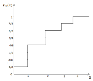
If X is a discrete random variable then the distribution function can be obtained by adding the probabilities successively.

Suppose X takes values x1,x2,…….,xn… with probabilities p(x1 ),p(x2 )……p(xn )….such that p(xi )=1, then by the definition of the distribution function FX (x) we have

FX (xi ) = p(X ≤ xi)

FX (xi ) = p(x1)+p(x2)+⋯…+p(xi)

So, for discrete random variable X, FX (x) is a monotonically increasing, right continuous, step function.

Figure 3. Discrete random variable

Key Take-Aways:

Cumulative distributive function
Probability density function
Properties of CDF and PDF

6.7 Statistical averages, mean, moments and expectations, Standard deviation and variance

Statistical Averages:

An average is defined as the number that measures the central tendency of a given set of numbers.

Mean

Mean refers to the number you obtain when you sum up a given set of numbers and then divide this sum by total number in the set. Mean is referred to more correctly as arithmetic mean

Mean = sum of elements in set / number of elements in set

Given a set of n elements from a1 to an

a1,a2, a3,a4 ……………………………………..an-1,an

Mean is found by adding all the a’s and then dividing the total number n

Mean = a1+a2+a3+a4+……………………..+an-1+an/n

This is generalized by the formula

Mean = 1/n

Example:

Find the mean of the set of numbers below

3,4,-1,22,14,0,9,18,7,0,1

Sum = 3+4+-1+22+14+0+9+18+7+0+1

Sum =77

Mean = sum/n

Mean = 77/10

Mean =7.7

Moments

Moments are a set of statistical parameters to measure a distribution. Four moments are commonly used:

1st, Mean: the average
2d, Variance:
- Standard deviation is the square root of the variance: an indication of how closely the values are spread about the mean. A small standard deviation means the values are all similar. If the distribution is normal, 63% of the values will be within 1 standard deviation.
3d, Skewness: measure the asymmetry of a distribution about its peak; it is a number that describes the shape of the distribution.
- It is often approximated by Skew = (Mean - Median) / (Std dev).
- If skewness is positive, the mean is bigger than the median and the distribution has a large tail of high values.
- If skewness is negative, the mean is smaller than the median and the distribution has a large tail of small values.
4th: Kurtosis: measures the peak or flatness of a distribution.
- Positive kurtosis indicates a thin pointed distribution.
- Negative kurtosis indicates a broad flat distribution.

Expectations:

The expectation of a random variable X is written as E(X). If we observe N random values of X, then the mean of the N values will be approximately equal to E(X) for large N.

In more concrete terms, the expectation is the expect the outcome of an experiment to be on an average if you repeat the experiment a large number of time.

If X is a continuous random variable with p.d.f Fx(x)

E[X] = FX(x) dx