Unit 1
INTRODUCTION – Well defined learning problems
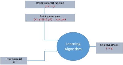
For any learning system, we must be knowing the three elements — T (Task), P (Performance Measure), and E (Training Experience). At a high level, the process of learning system looks as below.
|
Figure 1 Learning process algorithm
The learning process starts with task T, performance measure P and training experience E and objective are to find an unknown target function. The target function is an exact knowledge to be learned from the training experience and its unknown. For example, in a case of credit approval, the learning system will have customer application records as experience and task would be to classify whether the given customer application is eligible for a loan. So in this case, the training examples can be represented as (x1,y1)(x2,y2)..(xn,yn) where X represents customer application details and y represents the status of credit approval.
Linear Algebra and Statistical learning theory
The goal of learning process is to design a learning system that follows the learning process, it requires to consider a few design choices. The design choices are used to decide the key components:
1. Kind of training experience
2. The exact type of knowledge to be learned (it involves Choosing Target Function). At initial stage, steps of target function are not known.
3. A detailed representation of target knowledge (Choosing a representation for the Target Function)
4. A learning mechanism (Choosing an approximation algorithm for the Target Function)
We will look into the checkers learning problem and apply the above design choices. For a checkers learning problem, the three elements will be,
1. Task T: To play checkers
2. Performance measure P: Total percent of the game won in the tournament.
3. Training experience E: A set of games played against itself
Training experience
During the design of the checker's learning system, the type of training experience available for a learning system will have a significant effect on the success or failure of the learning.
- Direct or Indirect training experience — In the case of direct training experience, an individual board states and correct move for each board state are given.
In case of indirect training experience, the move sequences for a game and the final result (win, lose or draw) are given for a number of games. How to assign credit or blame to individual moves is the credit assignment problem.
2. Teacher or Not — Supervised — The training experience will be labelled, which means, all the board states will be labelled with the correct move. So the learning takes place in the presence of a supervisor or a teacher.
Unsupervised — The training experience will be unlabelled, which means, all the board states will not have the moves. So the learner generates random games and plays against itself with no supervision or teacher involvement.
Semi-supervised — Learner generates game states and asks the teacher for help in finding the correct move if the board state is confusing.
3. Is the training experience good — Do the training examples represent the distribution of examples over which the final system performance will be measured.
Performance is best when training examples and test examples are from the same/a similar distribution.
The checker player learns by playing against oneself. Its experience is indirect. It may not encounter moves that are common in human expert play. Once the proper training experience is available, the next design step will be choosing the Target Function.
Choosing the Target Function
In this design step, we need to determine exactly what type of knowledge has to be learned and it's used by the performance program.
When you are playing the checkers game, at any moment of time, you make a decision on choosing the best move from different possibilities. You think and apply the learning that you have gained from the experience. Here the learning is, for a specific board, you move a checker such that your board state tends towards the winning situation. Now the same learning has to be defined in terms of the target function.
Here there are 2 considerations — direct and indirect experience.
During the direct experience, the checkers learning system, it needs only to learn how to choose the best move among some large search space. We need to find a target function that will help us choose the best move among alternatives. Let us call this function ChooseMove and use the notation.
ChooseMove : B →M to indicate that this function accepts as input any board from the set of legal board states B and produces as output some move from the set of legal moves M.
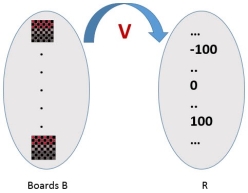
When there is an indirect experience, it becomes difficult to learn such function. How about assigning a real score to the board state. So the function be V : B →R indicating that this accepts as input any board from the set of legal board states B and produces an output a real score. This function assigns the higher scores to better board states.
|
Figure 2
If the system can successfully learn such a target function V, then it can easily use it to select the best move from any board position.
Let us therefore define the target value V(b) for an arbitrary board state b in B, as follows:
1. if b is a final board state that is won, then V(b) = 100 2. if b is a final board state that is lost, then V(b) = -100 3. if b is a final board state that is drawn, then V(b) = 0 4. if b is a not a final state in the game, then V (b) = V (b’), where b’ is the best final board state that can be achieved starting from b and playing optimally until the end of the game. |
The (4) is a recursive definition and to determine the value of V(b) for a particular board state, it performs the search ahead for the optimal line of play, all the way to the end of the game. So, this definition is not efficiently computable by our checkers playing program, we say that it is a non-operational definition.
The goal of learning, in this case, is to discover an operational description of V; that is, a description that can be used by the checkers-playing program to evaluate states and select moves within realistic time bounds.
It may be very difficult in general to learn such an operational form of V perfectly. We expect learning algorithms to acquire only some approximation to the target function ^V.
Choosing a representation for the Target Function
Now it’s time to choose a representation that the learning program will use to describe the function ^V that it will learn. The representation of ^V can be as follows.
- A table specifying values for each possible board state?
- collection of rules?
- neural network?
- a polynomial function of board features
To keep the discussion simple, let us choose a simple representation for any given board state, the function ^V will be calculated as a linear combination of the following board features:
^V = w0 + w1 · x1(b) + w2 · x2(b) + w3 · x3(b) + w4 · x4(b) +w5 · x5(b) + w6 · x6(b) |
Where w0 through w6 are numerical coefficients or weights to be obtained by a learning algorithm. Weights w1 to w6 will determine the relative importance of different board features.
Specification of the Machine Learning Problem at this time — Till now we worked on choosing the type of training experience, choosing the target function and its representation. The checkers learning task can be summarized as below.
Task T : Play Checkers Performance Measure : % of games won in world tournament Training Experience E : opportunity to play against itself Target Function : V : Board → R Target Function Representation : ^V = w0 + w1 · x1(b) + w2 · x2(b) + w3 · x3(b) + w4 · x4(b) +w5 · x5(b) + w6 · x6(b) |
The first three items above correspond to the specification of the learning task, whereas the final two items constitute design choices for the implementation of the learning program.
Choosing an approximation algorithm for the Target Function
Generating training data —
To train our learning program, we need a set of training data, each describing a specific board state b and the training value V_train (b) for b. Each training example is an ordered pair <b,V_train(b)> For example, a training example may be <(x1 = 3, x2 = 0, x3 = 1, x4 = 0, x5 = 0, x6 = 0), +100">. This is an example where black has won the game since x2 = 0 or red has no remaining pieces. However, such clean values of V_train (b) can be obtained only for board value b that are clear win, lose or draw. |
In above case, assigning a training value V_train(b) for the specific boards b that are clean win, lose or draw is direct as they are direct training experience. But in the case of indirect training experience, assigning a training value V_train(b) for the intermediate boards is difficult. In such case, the training values are updated using temporal difference learning. Temporal difference (TD) learning is a concept central to reinforcement learning, in which learning happens through the iterative correction of your estimated returns towards a more accurate target return.
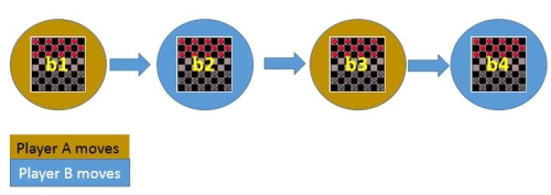
Let Successor(b) denotes the next board state following b for which it is again the program’s turn to move. ^V is the learner’s current approximation to V. Using this information, assign the training value of V_train(b) for any intermediate board state b as below:
V_train(b) ← ^V(Successor(b))
|
Figure 3
In the above figure, V_train(b1) ← ^V(b3), where b3 is the successor of b1. Once the game is played, the training data is generated. For each training example, the V_train(b) is computed.
Adjusting the weights
Now its time to define the learning algorithm for choosing the weights and best fit the set of training examples. One common approach is to define the best hypothesis as that which minimizes the squared error E between the training values and the values predicted by the hypothesis ^V.
|
The learning algorithm should incrementally refine weights as more training examples become available and it needs to be robust to errors in training data
Least Mean Square (LMS) training rule is the one training algorithm that will adjust weights a small amount in the direction that reduces the error.
The LMS algorithm is defined as follows:
|
Final Design for Checkers Learning system
- The performance System — Takes a new board as input and outputs a trace of the game it played against itself.
- The Critic — Takes the trace of a game as an input and outputs a set of training examples of the target function.
- The Generalizer — Takes training examples as input and outputs a hypothesis that estimates the target function. Good generalization to new cases is crucial.
- The Experiment Generator — Takes the current hypothesis (currently learned function) as input and outputs a new problem (an initial board state) for the performance system to explore
Issues in Machine Learning
Key Takeaways
- For any learning system, we must be knowing the three elements — T (Task), P (Performance Measure), and E (Training Experience).
- The learning process starts with task T, performance measure P and training experience E and objective are to find an unknown target function.
- The goal of learning process is to design a learning system that follows the learning process, it requires to consider a few design choices.
- learning has to be defined in terms of the target function.
- Here there are 2 considerations — direct and indirect experience.
- the function ^V will be calculated as a linear combination of the board features.
The Learning Task
Given: Instances X: set of items over which the concept is defined. Hypotheses H: conjunction of constraints on attributes. Target concept c: c : X → {0, 1} Training examples (positive/negative): <x,c(x)> Training set D: available training examples Determine: i A hypothesis h in H such that h(x) = c(x), for all x in X |
1.2.1. General-to-specific ordering of hypotheses
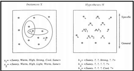
More_general_than_or_equal_to relation hj ≥ g hk ⇔ (∀x∈X)[(hk(x) =1)→(hj(x) =1)] (Strictly) more_general_than relation
<Sunny,?,?,?,?,?> >g <Sunny,?,?,Strong,?,?>
|
More_General_Than Relation
|
Figure 4
Find-S: Finding a Maximally Specific Hypothesis
1. Initialize h to the most specific hypothesis in H
2. For each positive training example x For each attribute constraint ai in h If the constraint ai is satisfied by x Then do nothing Else replace ai in h by the next more general constraint satisfied by x
3. Output hypothesis h
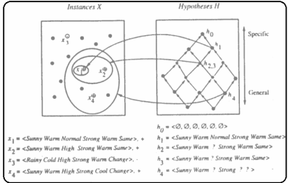
Hypothesis Space Search by Find-S
Properties of Find-S Ignores every negative example (no revision to h required in response to negative examples). Why? What’re the assumptions for this? Guaranteed to output the most specific hypothesis consistent with the positive training examples (for conjunctive hypothesis space). Final h also consistent with negative examples provided the target c is in H and no error in D
|
Figure 5
The List-Then-Eliminate algorithm initializes the version space to contain all hypotheses in H, then eliminates the hypotheses that are inconsistent, from training examples. The version space of hypotheses thus shrinks as more examples are observed until one hypothesis remains that is consistent with all the observed examples.
Presumably, this hypothesis is the desired target concept. If the data available is insufficient, to narrow the version space to a single hypothesis, then the algorithm can output the entire set of hypotheses consistent with the observed data.
The List-Then-Eliminate algorithm can be applied whenever the hypothesis space “H” is finite.
It has many advantages, including the fact that it is guaranteed to output all hypotheses consistent with the training data.
It requires exhaustively enumerating all hypotheses in H — an unrealistic requirement for all but the most trivial hypothesis spaces.
|
1.2.2 Inductive bias
Inductive bias refers to the restrictions that are imposed by the assumptions made in the learning method.
For example, assuming that the solution to the problem of road safety can be expressed as a conjunction of a set of eight concepts. This does not allow for more complex expressions that cannot be expressed as conjunction.
This inductive bias means that there are some potential solutions that we cannot explore, and not contained within the version space we examine.
In order to have an unbiased learner, the version space would have to contain every possible hypothesis that could possibly be expressed.
The solution that the learner produced could never be more general than the complete set of training data.
In other words, it would be able to classify data that it had previously seen (as the rote learner could) but would be unable to generalize in order to classify new, unseen data.
The inductive bias of the candidate elimination algorithm is that it is only able to classify a new piece of data if all the hypotheses contained within its version space give data the same classification. Hence, the inductive bias does not impose a limitation on the learning method
CE: Candidate-Elimination Algorithm
- Initialize G to the set of maximally general hypotheses in H
- Initialize S to the set of maximally specific hypotheses in H
- For each training example d, do
- If d is a positive example
- Remove from G any hypothesis inconsistent with d
- For each hypothesis s in S that is not consistent with d
- Remove s from S
- Add to S all minimal generalizations h of s such that
- h is consistent with d, and some member of G is more general
- than h
- Remove from S any hypothesis that is more general than another
- hypothesis in S
Candidate-Elimination Algorithm part 2
- If d is a negative example
- Remove from S any hypothesis inconsistent with d
- For each hypothesis g in G that is not consistent with d
- Remove g from G
- Add to G all minimal specializations h of g such that
- h is consistent with d, and some member of S is more specific than h
- Remove from G any hypothesis that is less general than another hypothesis in G
1.2.3 Evaluation and cross validation
Evaluation Techniques
We can evaluate the performance of a machine learning model, which is an integral component of any data science project. Model evaluation aims to estimate the generalization accuracy of a model on future (unseen/out-of-sample) data.
Methods for evaluating a model’s performance are divided into 2 categories: namely, holdout and Cross-validation. Both methods use a test set (i.e data not seen by the model) to evaluate model performance. It’s not recommended to use the data we used to build the model to evaluate it. This is because our model will simply remember the whole training set, and will therefore always predict the correct label for any point in the training set. This is known as overfitting.
Holdout
The purpose of holdout evaluation is to test a model on different data than it was trained on. This provides an unbiased estimate of learning performance.
In this method, the dataset is randomly divided into three subsets:
- Training set is a subset of the dataset used to build predictive models.
- Validation set is a subset of the dataset used to assess the performance of the model built in the training phase. It provides a test platform for fine-tuning a model’s parameters and selecting the best performing model. Not all modelling algorithms need a validation set.
- Test set, or unseen data, is a subset of the dataset used to assess the likely future performance of a model. If a model fits to the training set much better than it fits the test set, overfitting is probably the cause.
The holdout approach is useful because of its speed, simplicity, and flexibility. However, this technique is often associated with high variability since differences in the training and test dataset can result in meaningful differences in the estimate of accuracy.
Cross-Validation
Cross-validation is a technique that involves partitioning the original observation dataset into a training set, used to train the model, and an independent set used to evaluate the analysis.
The most common cross-validation technique is k-fold cross-validation, where the original dataset is partitioned into k equal size subsamples, called folds. The k is a user-specified number, usually with 5 or 10 as its preferred value. This is repeated k times, such that each time, one of the k subsets is used as the test set/validation set and the other k-1 subsets are put together to form a training set. The error estimation is averaged over all k trials to get the total effectiveness of our model.
For instance, when performing five-fold cross-validation, the data is first partitioned into 5 parts of (approximately) equal size. A sequence of models is trained. The first model is trained using the first fold as the test set, and the remaining folds are used as the training set. This is repeated for each of these 5 splits of the data and the estimation of accuracy is averaged over all 5 trials to get the total effectiveness of our model.
As can be seen, every data point gets to be in a test set exactly once and gets to be in a training set k-1 time. This significantly reduces bias, as we’re using most of the data for fitting, and it also significantly reduces variance, as most of the data is also being used in the test set. Interchanging the training and test sets also adds to the effectiveness of this method.
1.2.4 Optimisation methods
Fundamental optimisation methods are typically categorised into first-order, high-order and derivative-free optimisation methods.
Gradient Descent
The gradient descent method is the most popular optimisation method. The idea of this method is to update the variables iteratively in the (opposite) direction of the gradients of the objective function. With every update, this method guides the model to find the target and gradually converge to the optimal value of the objective function.
Conjugate Gradient Method
The conjugate gradient (CG) approach is used for solving large scale linear systems of equations and nonlinear optimisation problems. The first-order methods have a slow convergence speed. Whereas, the second-order methods are resource-heavy. Conjugate gradient optimisation is an intermediate algorithm, which combines the advantages of first-order information while ensuring the convergence speeds of high-order methods.
Key Takeaways
- Concept learning is Acquiring the definition of a general category given a sample of positive and negative training examples of the category and Inferring a Boolean-valued function from training examples of its input and output.
- The List-Then-Eliminate algorithm initializes the version space to contain all hypotheses in H, then eliminates the hypotheses that are inconsistent, from training examples.
- Properties of Find-S Ignores every negative example (no revision to h required in response to negative examples).
- Developers always use ML to develop predictors. Such predictors include improving search results and product selections and anticipating the behaviour of customers
- ML algorithms can pinpoint the specific biases which can cause problems for a business.
References
- Machine Learning. Tom Mitchell. First Edition, McGraw- Hill, 1997
- Introduction to Machine Learning Edition 2, by Ethem Alpaydin
- Suggested Reference Books:
- J. Shavlik and T. Dietterich (Ed), Readings in Machine Learning, Morgan Kaufmann, 1990.
- P. Langley, Elements of Machine Learning, Morgan Kaufmann, 1995.
- Understanding Machine Learning. Shai Shalev-Shwartz and Shai Ben-David. Cambridge
- University Press. 2017. [SS-2017]
- The Elements of Statistical Learning. Trevor Hastie, Robert Tibshirani and Jerome Friedman. Second Edition. 2009. [TH-2009]
