Unit 3

Classification & Regression

3.1 Linear Classification, Logistic Regression, Linear Discriminant Analysis, Quadratic Discriminant Analysis

Linear classifiers classify data into labels based on a linear combination of input features. Therefore, these classifiers separate data using a line or plane or a hyperplane (a plane in more than 2 dimensions). They can only be used to classify data that is linearly separable. They can be modified to classify non-linearly separable data

We will explore 3 major algorithms in linear binary classification -

Perceptron

In Perceptron, we take weighted linear combination of input features and pass it through a thresholding function which outputs 1 or 0. The sign of wTx tells us which side of the plane wTx=0, the point x lies on. Thus, by taking threshold as 0, perceptron classifies data based on which side of the plane the new point lies on.

The task during training is to arrive at the plane (defined by w) that accurately classifies the training data. If the data is linearly separable, perceptron training always converges

Logistic Regression

In Logistic regression, we take weighted linear combination of input features and pass it through a sigmoid function which outputs a number between 1 and 0. Unlike perceptron, which just tells us which side of the plane the point lies on, logistic regression gives a probability of a point lying on a particular side of the plane. The probability of classification will be very close to 1 or 0 as the point goes far away from the plane. The probability of classification of points very close to the plane is close to 0.5

SVM

There can be multiple hyperplanes that separate linearly separable data. SVM calculates the optimal separating hyperplane using concepts of geometry.

Linear Discriminant Analysis (LinearDiscriminantAnalysis) and Quadratic Discriminant Analysis (QuadraticDiscriminantAnalysis) are two classic classifiers, with, as their names suggest, a linear and a quadratic decision surface, respectively.

These classifiers are attractive because they have closed-form solutions that can be easily computed, are inherently multiclass, have proven to work well in practice, and have no hyperparameters to tune.

Properties of LDA

LDA has the following properties:

• LDA assumes that the data are Gaussian. More specifically, it assumes that all classes share the same covariance matrix.
• LDA finds linear decision boundaries in a K−1K−1 dimensional subspace. As such, it is not suited if there are higher-order interactions between the independent variables.
• LDA is well-suited for multi-class problems but should be used with care when the class distribution is imbalanced because the priors are estimated from the observed counts. Thus, observations will rarely be classified to infrequent classes.
• Similarly, to PCA, LDA can be used as a dimensionality reduction technique. Note that the transformation of LDA is inherently different to PCA because LDA is a supervised method that considers the outcomes.

3.2 Perceptron, Support Vector Machines

Perceptron is a single layer neural network and a multi-layer perceptron is called Neural Networks.

Perceptrons

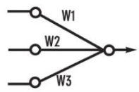
A perceptron is a neural network unit (an artificial neuron) that does certain computations to detect features or business intelligence in the input data.

A Perceptron can also be explained as an algorithm for supervised learning of binary classifiers. it enables neurons to learn and processes elements in the training set one at a time.

Figure 1

There are two types of Perceptrons:

• Single layer Perceptrons can learn only linearly separable patterns.
• Multilayer Perceptrons or feedforward neural networks with two or more layers have the greater processing power.

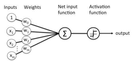
The Perceptron algorithm learns the weights for the input signals in order to draw a linear decision boundary.

Figure 2

Perceptron Learning Rule

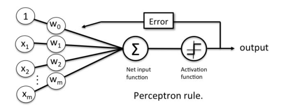
Perceptron Learning Rule states that the algorithm would automatically learn the optimal weight coefficients. The input features are then multiplied with these weights to determine if a neuron fires or not.

The Perceptron receives multiple input signals, and if the sum of the input signals exceeds a certain threshold, it either outputs a signal or does not return an output. In the context of supervised learning and classification, this can then be used to predict the class of a sample.

Figure 3

Gradient descent and the Delta rule

Gradient descent is an optimization algorithm used to find the values of parameters (coefficients) of a function (f) that minimizes a cost function (cost). It is best used when the parameters cannot be calculated analytically (e.g., using linear algebra) and must be searched for by an optimization algorithm.

Types of gradient descent:

•         Batch gradient descent refers to calculating the derivative from all training data before calculating an update.

•         Stochastic gradient descent refers to calculating the derivative from each training data instance and calculating the update immediately

Generalized Delta Learning Rule

Delta rule works only for the output layer. On the other hand, generalized delta rule, also called as back-propagation rule, is a way of creating the desired values of the hidden layer.

The Delta Rule uses the difference between target activation (i.e., target output values) and obtained activation to drive learning.

Terms used in delta rule:

 Threshold activation function & instead a linear sum of products is used to calculate the activation of the output neuron (alternative activation functions can also be applied). That’s why the activation function is called a Linear Activation function, in which the output node’s activation is simply equal to the sum of the network’s respective input/weight products.

The strength of network connections (i.e., the values of the weights) are adjusted to reduce the difference between target and actual output activation (i.e., error). delta rule can be summarized as:

Adaline, Multilayer networks

Both Adaline and Perceptron are neural network models of single-layer. Perceptron is oldest and simplest learning algorithms.

Adaline and the Perceptron have similarities:

• Act as classifiers for binary classification
• both have a linear decision boundary
• can learn iteratively, sample by sample (the Perceptron naturally, and Adaline via stochastic gradient descent)
• both use a threshold function

though Adaline requires continuous predicted values taken from net input to learn the model coefficients, which is more efficient as it can measure the accuracy of our selection.

Support Vector Machine or SVM is one of the most popular Supervised Learning algorithms, which is used for Classification as well as Regression problems. However, primarily, it is used for Classification problems in Machine Learning.

The goal of the SVM algorithm is to create the best line or decision boundary that can segregate n-dimensional space into classes so that we can easily put the new data point in the correct category in the future. This best decision boundary is called a hyperplane.

SVM chooses the extreme points/vectors that help in creating the hyperplane. These extreme cases are called as support vectors, and hence algorithm is termed as Support Vector Machine. Consider the below diagram in which there are two different categories that are classified using a decision boundary or hyperplane:

Types of SVM

SVM can be of two types:

• Linear SVM: Linear SVM is used for linearly separable data, which means if a dataset can be classified into two classes by using a single straight line, then such data is termed as linearly separable data, and classifier is used called as Linear SVM classifier.
• Non-linear SVM: Non-Linear SVM is used for non-linearly separated data, which means if a dataset cannot be classified by using a straight line, then such data is termed as non-linear data and classifier used is called as Non-linear SVM classifier.

Supervised Machine Learning:

Supervised learning is a machine learning method in which models are trained using labelled data. In supervised learning, models need to find the mapping function to map the input variable (X) with the output variable (Y).

Y= f( X)

Supervised learning needs supervision to train the model, which is similar to as a student learns things in the presence of a teacher. Supervised learning can be used for two types of problems: Classification and Regression.

Unsupervised Machine Learning:

Unsupervised learning is another machine learning method in which patterns inferred from the unlabelled input data. The goal of unsupervised learning is to find the structure and patterns from the input data. Unsupervised learning does not need any supervision. Instead, it finds patterns from the data by its own.

Unsupervised learning can be used for two types of problems: Clustering and Association.

Example: To understand the unsupervised learning, we will use the example given above. So unlike supervised learning, here we will not provide any supervision to the model. We will just provide the input dataset to the model and allow the model to find the patterns from the data. With the help of a suitable algorithm, the model will train itself and divide the fruits into different groups according to the most similar features between them.

The main differences between Supervised and Unsupervised learning are given below:

Key Takeaways

1. Machine learning, specifically supervised learning, can be described as the desire to use available data to learn a function that best maps inputs to outputs.
2. A common notation is used where lowercase-h (h) represents a given specific hypothesis and uppercase-h (H) represents the hypothesis space that is being searched.
3. supervised learning algorithms are trained using labeled data.
4. Unsupervised learning algorithms are trained using unlabeled data.
5. Methods and Types of sampling:
   • Simple Random Sampling
   • Systematic Sampling
   • Stratified Sampling

3.1.2 Kernels, Artificial Neural Networks, Back Propagation, Decision Trees, Bayes Optimal Classifier, Naive Bayes.

KERNELS

a kernel function measures the similarity between two data points. The notion of similarity is task-dependent. So, for instance, if your task is object recognition, then a good kernel will assign a high score to a pair of images that contain the same objects, and a low score to a pair of images with different objects.

Note that such a kernel captures much more abstract notion of similarity, compared to a similarity function that just compares two images pixel-by-pixel. As another example, consider a text processing task.

There, a good kernel function would assign high score to a pair of similar strings, and low score to a pair of dissimilar strings. This is the advantage of kernel functions — they can, in principle, capture arbitrarily complex notions of similarity, which can be used in various ML algorithms.

ARTIFICIAL NEURAL NETWORKS

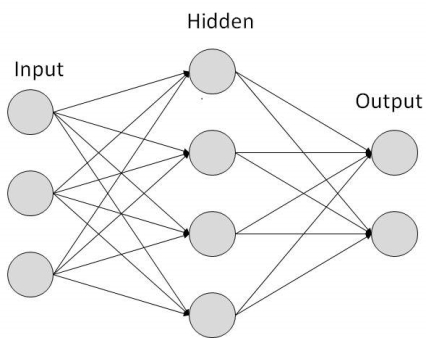
Neural networks are mathematical models that use learning algorithms inspired by the brain to store information. Since neural networks are used in machines, they are collectively called an ‘artificial neural network.’

Figure 4

Nowadays, the term machine learning is often used in this field and is the scientific discipline that is concerned with the design and development of algorithms that allow computers to learn, based on data, such as from sensor data or databases. A major focus of machine-learning research is to automatically learn to recognize complex patterns and make intelligent decisions based on data. Hence, machine learning is closely related to fields such as statistics, data mining, pattern recognition, and artificial intelligence. 

Neural networks are a popular framework to perform machine learning, but there are many other machine-learning methods, such as logistic regression, and support vector machines.

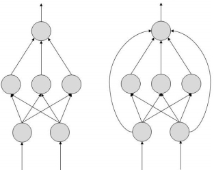
Types of Artificial Neural Networks

• FeedForward
• Feedback.

FeedForward ANN

In this ANN:

• information flow is unidirectional
• A unit sends information to other unit from which it does not receive any information.
• No feedback loops.
•  Used in pattern generation/recognition/classification.
• Have fixed inputs and outputs.

Figure 5

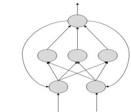
FeedBack ANN

• feedback loops are allowed.
•  used in content addressable memories.

Figure 6

Derivation of back propagation rule Back propagation Algorithm Convergence

The Backpropagation Algorithm is based on generalizing the Widrow-Hoff learning rule. It uses supervised learning, which means that the algorithm is provided with examples of the inputs and outputs that the network should compute, and then the error is calculated.

 The backpropagation algorithm starts with random weights, and the goal is to adjust them to reduce this error until the ANN learns the training data.

 Standard backpropagation is a gradient descent algorithm in which the network weights are moved along the negative of the gradient of the performance function. The combination of weights that minimizes the error function is considered a solution to the learning problem.

The backpropagation algorithm requires a differentiable activation function, and the most commonly used are tan-sigmoid, log-sigmoid, and, occasionally, linear. Feed-forward networks often have one or more hidden layers of sigmoid neurons followed by an output layer of linear neurons. This structure allows the network to learn nonlinear and linear relationships between input and output vectors. The linear output layer lets the network get values outside the range − 1 to + 1.

For the learning process, the data must be divided in two sets:

• training data set, which is used to calculate the error gradients and to update the weights;
• Validation data set, which allows selecting the optimum number of iterations to avoid overlearning.

 As the number of iterations increases, the training error reduces whereas the validation data set error begins to drop, then reaches a minimum and finally increases. Continuing the learning process after the validation error arrives at a minimum lead to overlearning. Once the learning process is finished, another data set (test set) is used to validate and confirm the prediction accuracy.

 Properly trained backpropagation networks tend to give reasonable answers when presented with new inputs. Usually, in ANN approaches, data normalization is necessary before starting the training process to ensure that the influence of the input variable in the course of model building is not biased by the magnitude of its native values, or its range of variation. The normalization technique, usually consists of a linear transformation of the input/output variables to the range (0, 1).

Feedforward Dynamics

When a BackPropagation network is cycled, the activations of the input units are propagated forward to the output layer through the connecting weights. As in perceptron, the net input to a unit is determined by the weighted sum of its inputs:

netj = iwjiai

where ai is the input activation from unit i and wji is the weight connecting unit i to unit j. However, instead of calculating a binary output, the net input is added to the unit's bias  and the resulting value is passed through a sigmoid function:

F(netj) = 1/(1 + e-netj+  j ).

The bias term plays the same role as the threshold in the perceptron. But unlike binary output of the perceptron, the output of a sigmoid is a continuous real-value between 0 and 1. The sigmoid function is sometimes called a "squashing" function because it maps its inputs onto a fixed range.

Naïve Bayes algorithm

The Naïve Bayes algorithm is comprised of two words Naïve and Bayes, which can be described as:

• Naïve: It is called Naïve because it assumes that the occurrence of a certain feature is independent of the occurrence of other features. Such as if the fruit is identified on the bases of colour, shape, and taste, then red, spherical, and sweet fruit is recognized as an apple. Hence each feature individually contributes to identify that it is an apple without depending on each other.
• Bayes: It is called Bayes because it depends on the principle of Bayes' Theorem.

Naïve Bayes Classifier Algorithm

Naïve Bayes algorithm is a supervised learning algorithm, which is based on Bayes theorem and used for solving classification problems. It is mainly used in text classification that includes a high-dimensional training dataset.

Naïve Bayes Classifier is one of the simple and most effective Classification algorithms which helps in building the fast machine learning models that can make quick predictions.

It is a probabilistic classifier, which means it predicts on the basis of the probability of an object.

Some popular examples of Naïve Bayes Algorithm are spam filtration, Sentimental analysis, and classifying articles.

Bayes' Theorem:

• Bayes' theorem is also known as Bayes' Rule or Bayes' law, which is used to determine the probability of a hypothesis with prior knowledge. It depends on the conditional probability.
• The formula for Bayes' theorem is given as:

Where,

P(A|B) is Posterior probability: Probability of hypothesis A on the observed event B.

P(B|A) is Likelihood probability: Probability of the evidence given that the probability of a hypothesis is true.

P(A) is Prior Probability: Probability of hypothesis before observing the evidence.

P(B) is Marginal Probability: Probability of Evidence.

Naïve Bayes classifier, Bayesian belief networks

Working of Naïve Bayes' Classifier:

Working of Naïve Bayes' Classifier can be understood with the help of the below example:

Suppose we have a dataset of weather conditions and corresponding target variable "Play". So, using this dataset we need to decide that whether we should play or not on a particular day according to the weather conditions. So to solve this problem, we need to follow the below steps:

Convert the given dataset into frequency tables.

Generate Likelihood table by finding the probabilities of given features.

Now, use Bayes theorem to calculate the posterior probability.

Problem: If the weather is sunny, then the Player should play or not?

Solution: To solve this, first consider the below dataset:

              Outlook Play

Frequency table for the Weather Conditions:

Likelihood table weather condition:

Applying Bayes' theorem:

So, as we can see from the above calculation that

P(Yes|Sunny)>P(No|Sunny)

Hence on a Sunny day, Player can play the game.

Advantages of Naïve Bayes Classifier:

Naïve Bayes is one of the fast and easy ML algorithms to predict a class of datasets.

It can be used for Binary as well as Multi-class Classifications.

It performs well in Multi-class predictions as compared to the other Algorithms.

It is the most popular choice for text classification problems.

Disadvantages of Naïve Bayes Classifier:

Naive Bayes assumes that all features are independent or unrelated, so it cannot learn the relationship between features.

Applications of Naïve Bayes Classifier:

It is used for Credit Scoring.

It is used in medical data classification.

It can be used in real-time predictions because Naïve Bayes Classifier is an eager learner.

It is used in Text classification such as Spam filtering and Sentiment analysis.

Types of Naïve Bayes Model:

There are three types of Naive Bayes Model, which are given below:

Gaussian: The Gaussian model assumes that features follow a normal distribution. This means if predictors take continuous values instead of discrete, then the model assumes that these values are sampled from the Gaussian distribution.

Multinomial: The Multinomial Naïve Bayes classifier is used when the data is multinomial distributed. It is primarily used for document classification problems, it means a particular document belongs to which category such as Sports, Politics, education, etc.

The classifier uses the frequency of words for the predictors.

Bernoulli: The Bernoulli classifier works similar to the Multinomial classifier, but the predictor variables are the independent Booleans variables. Such as if a particular word is present or not in a document. This model is also famous for document classification tasks.

Key Takeaways

1. Naïve: It is called Naïve because it assumes that the occurrence of a certain feature is independent of the occurrence of other features.
2. Bayes: It is called Bayes because it depends on the principle of Bayes' Theorem.
3. The formula for Bayes' theorem is given as:

References

1. Machine Learning. Tom Mitchell. First Edition, McGraw- Hill, 1997
2. Introduction to Machine Learning Edition 2, by Ethem Alpaydin
3. Suggested Reference Books:

• J. Shavlik and T. Dietterich (Ed), Readings in Machine Learning, Morgan Kaufmann, 1990.
• P. Langley, Elements of Machine Learning, Morgan Kaufmann, 1995.
• Understanding Machine Learning. Shai Shalev-Shwartz and Shai Ben-David. Cambridge University Press. 2017. [SS-2017]
• The Elements of Statistical Learning. Trevor Hastie, Robert Tibshirani and Jerome Friedman. Second Edition. 2009. [TH-2009]