Unit 5

Expectation Maximization

5.1 Expectation Maximization

The Expectation-Maximization (EM) algorithm is a way to find maximum-likelihood estimates for model parameters when your data is incomplete, has missing data points, or has unobserved (hidden) latent variables. It is an iterative way to approximate the maximum likelihood function. While maximum likelihood estimation can find the “best fit” model for a set of data, it doesn’t work particularly well for incomplete data sets.

The more complex EM algorithm can find model parameters even if you have missing data. It works by choosing random values for the missing data points, and using those guesses to estimate a second set of data. The new values are used to create a better guess for the first set, and the process continues until the algorithm converges on a fixed point.

Algorithm:

1. Given a set of incomplete data, consider a set of starting parameters.
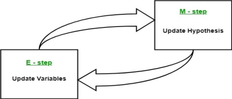
2. Expectation step (E – step): Using the observed available data of the dataset, estimate (guess) the values of the missing data.
3. Maximization step (M – step): Complete data generated after the expectation (E) step is used in order to update the parameters.
4. Repeat step 2 and step 3 until convergence.

Figure 1

The essence of Expectation-Maximization algorithm is to use the available observed data of the dataset to estimate the missing data and then using that data to update the values of the parameters. Let us understand the EM algorithm in detail.

• Initially, a set of initial values of the parameters are considered. A set of incomplete observed data is given to the system with the assumption that the observed data comes from a specific model.
• The next step is known as “Expectation” – step or E-step. In this step, we use the observed data in order to estimate or guess the values of the missing or incomplete data. It is basically used to update the variables.
• The next step is known as “Maximization”-step or M-step. In this step, we use the complete data generated in the preceding “Expectation” – step in order to update the values of the parameters. It is basically used to update the hypothesis.
• Now, in the fourth step, it is checked whether the values are converging or not, if yes, then stop otherwise repeat step-2 and step-3 i.e., “Expectation” – step and “Maximization” – step until the convergence occurs.

Applications

The EM algorithm has many applications, including:

• Dis-entangling superimposed signals,
• Estimating Gaussian mixture models (GMMs),
• Estimating hidden Markov models (HMMs),
• Estimating parameters for compound Dirichlet distributions,
• Finding optimal mixtures of fixed models.

Limitations

The EM algorithm can be very slow, even on the fastest computer. It works best when you only have a small percentage of missing data and the dimensionality of the data isn’t too big. The higher the dimensionality, the slower the E-step; for data with larger dimensionality, you may find the E-step runs extremely slow as the procedure approaches a local maximum.

5.2 GMMs, Learning theory Intro to Reinforcement Learning

GA’s are adaptive heuristic search algorithms inspired by evolutionary algorithms. Genetic algorithms are based on the ideas of natural selection and genetics. It uses intelligent exploitation of random search provided with historical data to direct the search into the region of better performance in solution space. 

GA is commonly used to generate high-quality solutions for optimization problems and search problems.

GA simulate natural selection process which means only species who can adapt to changes in their environment are able to survive and reproduce and pass on to next generation.

 In simple words, they follow the principle of “survival of the fittest” among individual of consecutive generation for solving a problem.

 Each generation consist of a population of individuals and each individual represents a point in search space and possible solution. Each individual is represented as a string of bits (character/integer/float). This string is analogous to the Chromosome.

Principle of Genetic Algorithm

Genetic algorithms are based on an analogy with genetic structure and behaviour of chromosome of the population. Following is the foundation of GAs based on this analogy –

1. Individual in population compete for resources and mate
2. Those individuals who are successful (fittest) then mate to create more offspring than others
3. Genes from “fittest” parent propagate throughout the generation, that is sometimes parents create offspring which is better than either parent.
4. Thus, each successive generation is more suited for their environment

Illustrative example

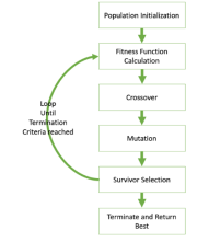
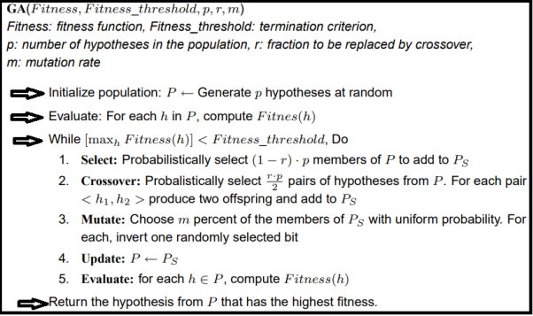
Figure 2 GA basic execution flow

Hypothesis space search

 Hypothesis method is not same as other methods presented till far. It is neither general-to-specific nor simple-to-complex. Search is performed genetic algorithms takes place in quick and undetermined way, replacing a parent hypothesis by an offspring which is radically different so this method is less likely to fall into some local minimum

Practical difficulty: crowding

 Some individuals that fit better than others reproduce quickly, so that copies and very similar offspring take over a large fraction of the population ⇒ reduced diversity of population ⇒ slower progress of the genetic algorithms

Hypotheses are often represented as bit strings so that they can easily be modified by genetic operators. The represented hypotheses can be quite complex as each attribute can be represented as a substring with a no. of positions. And as there are possible values to obtain a fixed-length bit string, each attribute has to be considered, even in the most general case.

Genetic Programming

Genetic programming (GP) is an evolutionary approach that exploits genetic algorithms to allow the exploration of the space of computer programs. GP works by defining a goal in the form of a quality criterion also known as fitness) and then using this criterion to evolve a set (or population) of candidate solutions by using the basic principles of Darwinian evolution. GP reproduces the solutions to problems using an iterative process involving the probabilistic selection of the fittest solutions and their variation by means of a set of genetic operators, usually crossover and mutation. GP has been successfully applied to a number of challenging real-world problem domains.

Its operations and behaviour are now reasonably well understood thanks to a variety of powerful theoretical results

Advantages of GAs

GAs have various advantages which have made them immensely popular. These include −

• Does not require any derivative information (which may not be available for many real-world problems).
• Is faster and more efficient as compared to the traditional methods.
• Has very good parallel capabilities.
• Optimizes both continuous and discrete functions and also multi-objective problems.
• Provides a list of “good” solutions and not just a single solution.
• Always gets an answer to the problem, which gets better over the time.
• Useful when the search space is very large and there are a large number of parameters involved.

Limitations of GAs

• not suited for problems which are simple and for which derivative information is available.
• Fitness value is calculated repeatedly which might be computationally expensive for some problems.
• Being stochastic, there are no guarantees on the optimality or the quality of the solution.
• If not implemented properly, the GA may not converge to the optimal solution.

Key Takeaways

1. GA’s are adaptive heuristic search algorithms inspired by evolutionary algorithms. Genetic algorithms are based on the ideas of natural selection and genetics.
2. Following is the foundation of GAs based on this analogy –
   • Individual in population compete for resources and mate
   • Those individuals who are successful (fittest) then mate to create more offspring than others
   • Genes from “fittest” parent propagate throughout the generation, that is sometimes parents create offspring which is better than either parent.
   • Thus, each successive generation is more suited for their environment.

REINFORCEMENT LEARNING - The Learning Task, Q Learning.

Reinforcement learning (RL) solves a particular kind of problem where decision making is sequential, and the goal is long-term, such as game playing, robotics, resource management, or logistics.

RL is an area of Machine Learning which is related to taking suitable action to maximize reward in a particular situation. It is employed by various software and machines to find the best possible behaviour or path. RL differs from the supervised learning in a way that the training data has the answer key with it so the model is trained with the correct answer itself whereas in reinforcement learning, there is no answer but reinforcement agent decides what to do to perform the given task. In the absence of a training dataset, it is bound to learn from its experience.

Example:

For a robot, an environment is a place where it has been put to use. Remember this robot is itself the agent. For example, a textile factory where a robot is used to move materials from one place to another.

These tasks have a property in common:

-  these tasks involve an environment and expect the agents to learn from that environment. This is where traditional machine learning fails and hence the need for reinforcement learning.

q-learning

Q-learning is another type of reinforcement learning algorithm that seeks to find the best action to take given the current state. It’s considered as the  off-policy because the q-learning function learns from actions that are outside the current policy, such as  taking random actions, and therefore a policy isn’t needed.

 More specifically, q-learning seeks to learn a policy that maximizes the total reward.

Role of ‘Q’

The ‘q’ in q-learning stands for quality. Quality in this case represents how useful a given action is in gaining some future reward.

Create a q-table

When q-learning is performed we create what’s called a q-table or matrix that follows the shape of [state, action] and we initialize our values to zero. We then update and store our q-values after an episode. This q-table becomes a reference table for our agent to select the best action based on the q-value.

Updating the q-table

The updates occur after each step or action and ends when an episode is done. Done in this case means reaching some terminal point by the agent. A terminal state for example can be anything like landing on a checkout page, reaching the end of some game, completing some desired objective, etc. The agent will not learn much after a single episode, but eventually with enough exploring (steps and episodes) it will converge and learn the optimal q-values or q-star (Q∗).

Here are the 3 basic steps:

1. Agent starts in a state (s1) takes an action (a1) and receives a reward (r1)
2. Agent selects action by referencing Q-table with highest value (max) OR by random (epsilon, ε)
3. Update q-values

5.3 Bayesian Networks.

Bayesian belief network is key computer technology for dealing with probabilistic events and to solve a problem which has uncertainty. We can define a Bayesian network as:

"A Bayesian network is a probabilistic graphical model which represents a set of variables and their conditional dependencies using a directed acyclic graph."

It is also called a Bayes network, belief network, decision network, or Bayesian model.

Bayesian networks are probabilistic, because these networks are built from a probability distribution, and also use probability theory for prediction and anomaly detection.

Real world applications are probabilistic in nature, and to represent the relationship between multiple events, we need a Bayesian network. It can also be used in various tasks including prediction, anomaly detection, diagnostics, automated insight, reasoning, time series prediction, and decision making under uncertainty.

Bayesian Network can be used for building models from data and experts opinions, and it consists of two parts:

• Directed Acyclic Graph
• Table of conditional probabilities.

The generalized form of Bayesian network that represents and solve decision problems under uncertain knowledge is known as an Influence diagram.

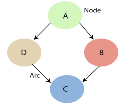
A Bayesian network graph is made up of nodes and Arcs (directed links), where:

Figure 4

Key Takeaways

1. Reinforcement learning (RL) solves a particular kind of problem where decision making is sequential, and the goal is long-term, such as game playing, robotics, resource management, or logistics.
2. The Bayesian network graph does not contain any cyclic graph. Hence, it is known as a directed acyclic graph or DAG.

References

1. Machine Learning. Tom Mitchell. First Edition, McGraw- Hill, 1997
2. Introduction to Machine Learning Edition 2, by Ethem Alpaydin
3. Suggested Reference Books:
   • J. Shavlik and T. Dietterich (Ed), Readings in Machine Learning, Morgan Kaufmann, 1990.
   • P. Langley, Elements of Machine Learning, Morgan Kaufmann, 1995.
   • Understanding Machine Learning. Shai Shalev-Shwartz and Shai Ben-David. Cambridge University Press. 2017. [SS-2017]
   • The Elements of Statistical Learning. Trevor Hastie, Robert Tibshirani and Jerome Friedman. Second Edition. 2009. [TH-2009]