Unit - 1

Solution of non-linear, linear equations and interpolation

1.1 Solution of non-linear equations in one variable: Bisection method

There are two types of equations Linear and Nonlinear equations. Linear equations are those in which dependent variable y is directly proportional to independent variable x and is of degree one. On the other hand, nonlinear equation is those in which y does not directly proportional to x and of degree more than one.

Ex: +b, where a and b are constant is a linear equation.

      is a non-linear equation.

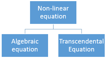
Algebraic Equation:

If f(x) is a pure polynomial, then the equation is called an algebraic equation in x.

Ex:

Transcendental Equation:

If f(x) is an expression contain function as trigonometric, exponential and logarithmic etc. Then is called transcendental equation.

Ex

Non –linear equation can be solved by using various analytical methods. The transcendental equations and higher order algebraic equations are difficult to solve even sometime are impossible. Finding solution of equation means just to calculate its roots.

Numerical methods are often repetitive in nature. They consist of repetitive calculation of the same process where in each step the result of preceding values are used (substitute).  This is known as iteration process and is repeated till the result is obtained to desired accuracy.

The analytical methods used to solve equation; exact value of the root is obtained whereas in numerical method approximate value is obtained.

Bisection method-

This method consists of finding the root of the equation    which lies between a and b (say).

The function is continuous function between a and b and f (a) and f (b) are of opposite signs then there is a least one root between a and b.

Suppose f (a) is negative and f (b) is positive, then the first approximate value of the root is                           

If, then the correct root is .But if, then the root either lies between a and or and b according as is positive or negative, we again bisect the interval as above and the process is repeated the root is found to desired accuracy.

Example:

Find a real root of using bisection method correct to five decimal places.

Let then by hit and trial we have

Thus .So the root of the given equation should lie between 1 and 2.

Now,

i.e., positive so the root of the given equation must lie between

Now,

i.e., negative so the root of the given equation lies between

Now,

i.e., positive so the root of the given equation lies between

Now,

i.e., negative so that the root of the given equation lies between

Now,

i.e., positive so that the root of the given equation lies between

Now,

i.e., positive so that the root of the given equation lies between

Now,

i.e. negative so that the root of the given equation lies between

Now,

i.e., negative so that the root of the given equation lies between

Hence the approximate root of the given equation is 1.32421

Example:

Find the root of the equation, using the bisection method.

Let then by hit and trial we have

Thus .So the root of the given equation should lie between 2 and 3.

Now,

i.e., negative so the root of the given equation must lie between

Now,

i.e., positive so the root of the given equation must lie between

Now,

i.e., negative so the root of the given equation must lie between

Now,

i.e., negative so the root of the given equation must lie between

Now,

i.e., positive so the root of the given equation must lie between

Now,

i.e., negative so the root of the given equation must lie between

Hence the root of the given equation correct to two decimal place is 2.67965.

Example3

Find the root of the equation   between 2 and 3, using bisection method correct to two decimal places.

Let

Where

Thus .So the root of the given equation should lie between 2 and 3.

Now,

i.e., positive so the root of the given equation must lie between

Now,

i.e., positive so the root of the given equation must lie between

Now,

i.e., negative so the root of the given equation must lie between

Now,

i.e., positive so the root of the given equation must lie between

Now,

i.e., positive so the root of the given equation must lie between

Now,

i.e., positive so the root of the given equation must lie between

Now,

i.e., positive so the root of the given equation must lie between

Now,

i.e., positive so the root of the given equation must lie between

Hence the root of the given equation correct to two decimal place is 2.1269

Key takeaways

1. Algebraic Equation- If f(x) is a pure polynomial, then the equation is called an algebraic equation in x.
2. Transcendental Equation- If f(x) is an expression contain function as trigonometric, exponential and logarithmic etc. Then is called transcendental equation.

1.2 Newton-Rapson method

Let be the approximate root of the equation.

By Newton Raphson formula

In general

Where n=1, 2, 3…… we keep on calculating until we get desired root to the correct decimal places.         

Example1 Using Newton-Raphson method, find a root of the following equation correct to 3 decimal places:.

Given

By Newton Raphson Method

= 

=

   The initial approximation is in radian.

      For n =0, the first approximation

For n =1, the second approximation

For n =2, the third approximation

For n =3, the fourth approximation

Hence the root of the given equation correct to five decimal place 2.79838.

Example2   Using Newton-Raphson method, find a root of the following equation correct to 3 decimal places: near to 4.5

Let

  The initial approximation

By Newton Raphson Method

     For n =0, the first approximation

  For n =1, the second approximation

For n =2, the third approximation

For n =3, the fourth approximation

     Hence the root of the equation correct to three decimal places is 4.5579

Example3 Using Newton-Raphson method, find a root of the following equation correct to 4 decimal places:

    Let

By Newton Raphson Method

Let the initial approximation be

For n=0, the first approximation

   For n=1, the second approximation

For n=2, the third approximation

Since therefore the root of the given equation correct to four decimal places is -2.9537

Key takeaways

1.3 Fixed point iteration method

The successive approximation is also known as iteration method. To start the solution using this method we need one or more approximate value which is not necessarily the root of the given equation.

We are finding the root of the given equation

       ... (1)

We rewrite the given equation in the form

     ... (2)

We know that the root of the equation lies between its positive and the negative values

Let 

So, the interval of the root of the equation be .

Now, let be an approximate root of the given equation (1).  

Putting it in equation (2) we get  

Successive substitution gives the approximations

…………..

If the above values converge to a definite   number, then that   number will be the root of the given equation.

Example1: Find the real root of the equation

Correct to three decimal places in the interval  ]

The given equation is      ... (1)

Or

Or =     ... (2)

Or

Let , in the interval .

The successive approximation we have

Hence the root of the equation correct to three decimal places is 1.524.

Example: Find the real root of the polynomial correct to three decimal places?

Given equation    …. (1)

      Here

Also

Therefore, root of the equation lies between .

Again

    …. (2)

Let , in the interval .

The successive approximation we have

Hence the root of the equation correct to three decimal places is 0.755.

Example3: By iteration method, find the value of , correct to three decimal places.

Let 

Let .

Also

Therefore, the root of the equation lies between 3 and 4.

Given equation can rewrite  .

Or … (2)

Let , in the interval .

The successive approximation we have

Hence the root of the equation correct to three decimal places is 3.634.

1.4 Numerical solution of system of linear equations: Guass-seidel method

Jacobi’s Iteration method:

Let us consider the system of simultaneous linear equation

The coefficients of the diagonal elements are larger than the all-other coefficients and are non-zero. Rewrite the above equation we get

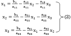
Take the initial approximation we get the values of the first approximation of .

By the successive iteration we will get the desired the result.

Example1 Use Jacobi’s method to solve the system of equations:

Since

So, we express the unknown with large coefficient in terms of other coefficients.

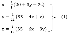
Let the initial approximation be

                                                        2.35606

                                                        0.91666

                                                        1.932936

                                                        0.831912

                                                      3.016873

                                                        1.969654

                                                      3.010217

                                                        1.986010

                                                        1.988631

                                                        0.915055

                                                        1.986532

                                                        0.911609

                                                        1.985792

                                                        0.911547

                                                        1.98576

                                                        0.911698

Since the approximation in ninth and tenth iteration is same up to three decimal places, hence the solution of the given equations is

Example2 Solve by Jacobi’s Method, the equations

Given equation can be rewrite in the form

                                         … (i)

                                        ...(ii)

                                         ...(iii)

Let the initial approximation be

Putting these values on the right of the equation (i), (ii) and (iii) and so we get

Putting these values on the right of the equation (i), (ii) and (iii) and so we get

Putting these values on the right of the equation (i), (ii) and (iii) and so we get

  0.90025

Putting these values on the right of the equation (i), (ii) and (iii) and so we get

Putting these values on the right of the equation (i), (ii) and (iii) and so we get

Hence   solution approximately is

Example3Use Jacobi’s method to solve the system of the equations

Rewrite the given equations

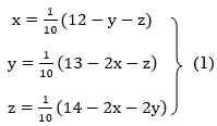
Let the initial approximation be

                                                              1.2

                                                            1.3

                                       0.9

                             1.03

                                                  0.9946

                                                  0.9934

                                         1.0015

Hence the solution of the above equation correct to two decimal places is

Gauss Seidel method:   

This is the modification of the Jacobi’s Iteration.  As above in Jacobi’s Iteration, we take first approximation as and put in the right-hand side of the first equation of (2) and let the result be  . Now we put right hand side of second equation of (2) and suppose the result is now put in the RHS of third equation of (2) and suppose the result be the above method is repeated till the values of all the unknown are found up to desired accuracy.

Example1 Use Gauss –Seidel Iteration method to solve the system of equations

Since

So, we express the unknown of larger coefficient in terms of the unknowns with smaller coefficients.

Rewrite the above system of equations

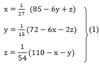
Let the initial approximation be

3.14814

2.43217

2.42571

2.4260

Hence the solution correct to three decimal places is

Example2 Solve the following system of equations

  By Gauss-Seidel method.

Rewrite the given system of equations as

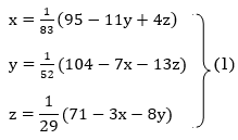
Let the initial approximation be

Thus, the required solution is

Example3 Solve the following equations by Gauss-Seidel Method

Rewrite the above system of equations

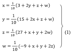
Let the initial approximation be

Hence the required solution is

1.5 Successive over relaxation and Doolittle method, Crouts and Choleskys method

LU decomposition method

The method is based on the fact that every matrix A can be expressed as the product of a lower triangular matrix and an upper triangular matrix.

This method is also known as the Triangularization method

In this method, the coefficient matrix A of the system of equations AX = B is decomposed into the product of a lower triangular matrix L and an upper triangular matrix U so that

Where

Using the matrix multiplication and comparing corresponding elements in (1), we obtain

Where

Now

In order to produce a unique solution, it is convenient to choose either

Note-

1. When we choose = 1, the method is called the Doolittle’s method.
2. When we choose = 1, the method is called the Crout’s method.

The given system of equations is

AX = B …… (2)

Using (1)

LUX = B…. (3)

Let UX = Y then equation (3)-

LY = B

 y1, y2, y3, ..., yn in (4) are fi by forward substitution and the unknowns x1, x2, x3, ..., xn in UX = Y are obtained by back substitution.

Note- The method fails if any of the diagonal elements or is zero.

Example: Solve the equations-

Sol.

Let

So that-

3.    

4.    

5.    

So

Thus-

Writing UX = V,

The system of given equations become-

By solving this-

We get-

Therefore, the given system becomes-

Which means-

By back substitution, we get the values of x, y and z

Example:

Solve by using Crout’s method, the following system of equations:

x + y + z = 3

2x – y + 3z = 16

3x + y – z = – 3

Sol:

Choosing

We get by equating

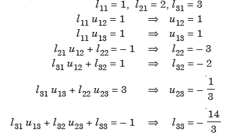
Thus, we get

The given system is

AX = B

LUX = B ... (1)

Let UX = Y so that (1) becomes

LY = B

Which gives

Now

UX = Y

Which gives,

x + y + z = 3

y – z/3 = -10/3

z = 4

By back substitution

X = 1, y = -2 and z = 4

Cholesky’s method

Consider a system of equations

AX = B … (1)

If the coefficient matrix A is symmetric and positive definite then A can be decomposed as

Where L is a lower triangular matrix.

A may also be decomposed as where U is an upper triangular matrix.

From (1) and (2),

Where

The values , 1 i n can be obtained by forward substitution and the solution ,,1 i n are obtained by back substitution.

Key takeaways

1. When we choose = 1, the method is called the Doolittle’s method.
2. When we choose = 1, the method is called the Crout’s method.
3. The method fails if any of the diagonal elements or is zero

1.6 Interpolation: Newton’s forward and backward interpolation

Interpolation

Definition:

Interpolation is a technique of estimating the value of a function for any intermediate value of the independent variable while the process of computing the value of the function outside the given range is called   extrapolation.

Let be a function of x.

The table given below gives corresponding values of y for different values of x.

X  ….

y= f(x)….

The process of finding the values of y corresponding to any value of x which lies between   is called interpolation.

If the given function is a polynomial, it is polynomial interpolation and given function is known as interpolating polynomial.

Note- The process of computing the value of the function outside the given range is called extrapolation.

Thus, interpolation is the “art of reading between the lines of a table.”

Conditions for Interpolation

1)     The function must be   a polynomial of independent variable.

2)     The function   should be either increasing or decreasing function.

3)     The value of   the function should be increase or decrease uniformly.

Finite Difference

Let be a function of x. The table given below gives corresponding values of y for different values of x.

X  ….

y= f(x)….

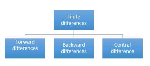
There are three types of differences are useful-

a)     Forward Difference: 
The  are called differences of y, denoted by 

The symbol   is called the forward difference operator.  Consider the forward difference table below:

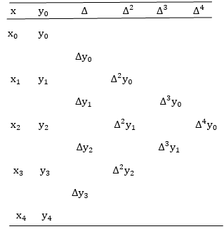
Where

   And third forward difference so on.

b)    Backward Difference:

The difference are called first backward difference and is denoted by  Consider the backward difference table below:

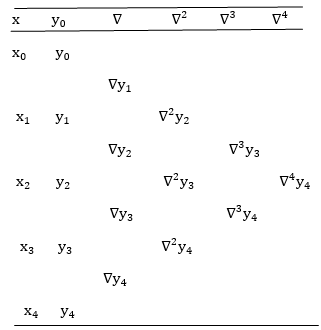
Where

And third backward differences so on.

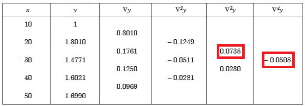
Example: Construct a backward difference table for y = log x, given-

Sol. The backward difference table will be-

Newton Forward Difference formula:

    This method is useful for interpolation near the beginning of a set of tabular values.

    Where

Example1: Using Newton’s forward difference formula, find the sum

Putting

It   follows that

Since is a fourth-degree polynomial in n.

Further,

By Newton Forward Difference Method

Example2: Given  find   , by using Newton forward interpolation method.

Let , then

	0.7071	0.7660	-	0.8192	0.8660

The table of forward finite difference is given below:

45           50           55            60	0.7071            0.7660           0.8192            0.8660	0.0589          0.0532          0.0468	-0.0057        -0.0064	-0.0007

By Newton forward difference method

Here initial value = 45, difference of interval h = 5 and the value to be calculated at x=52.

By Formula

Example3: Find the missing term in the following:

	0	1	2	3	4
	1	3	9	?	81

Let

First, we construct the forward difference table:

0       1        2        3        4	1       3       9             81	2         6	4

Now,

Newton Backward Difference Method:

This method is useful for interpolation near the ending of a set of tabular values.

Where 

Example1:  Find from the following table:

	0.20	0.22	0.24	0.26	0.28	0.30
	1.6596	1.6698	1.6804	1.6912	1.7024	1.7139

Consider the backward difference method

0.20         0.22         0.24         0.26         0.28         0.30	1.6596      1.6698      1.6804      1.6912     1.7024       1.7139	0.0102       0.0106      0.0108      0.0112     0.0115	0.0004   0.0002   0.0004   0.0003	-0.0002   0.0002   -0.0001	0.0004   -0.0003	-0.0007

  Here

By Newton backward difference formula

Example2: The following table give the amount of a chemical dissolved in water:

Temp.
Solubility	19.97	21.51	22.47	23.52	24.65	25.89

  Compute the amount dissolve at

Consider the following backward difference table:

Temp.  x	Solubility y
10     15     20     25     30     35	19.97      21.51     22.47     23.52      24.65      25.89	1.54     0.96   1.05     1.13     1.24	-0.58      0.09      0.08      0.11	0.67     -0.01      0.03	-0.68     0.04	0.72

Here

   By Newton Backward difference formula

Example3: The following are the marks obtained by 492 candidates in a certain examination

Find out the number of candidates:

a)     Who secured more than 48 but not more than 50 marks?

b)    Who secured less than 48 but not less than 45 marks?

Consider the forward difference table given below:

Marks up to x	No. Of candidates y
40       45       50       55       60       65	210   210+43=253   253+54=307   307+74=381   381+32=413   413+79= 492	43       54       74       32        79	11     20     -42      47	9     -62      89	-71        151	222

               Here 

By Newton Forward Difference formula

f

a)     No. Of candidate secured more than 48 but not more than 50 marks

b)    No. Of candidate secured less than 48 but not less than 45 marks

Key takeaways-

1. Interpolation is a technique of estimating the value of a function for any intermediate value of the independent variable while the process of computing the value of the function outside the given range is called   extrapolation.
2. If the given function is a polynomial, it is polynomial interpolation and given function is known as interpolating polynomial.

c)     Forward Difference:  The  are called differences of y, denoted by 

The symbol  is called the forward difference operator

3.     Backward Difference:

The difference are called first backward difference and is denoted by 

1. Newton Forward Difference formula:

    Where

2.     Newton Backward Difference Method:

Where 

1.7 Newton’s divided difference interpolation

Divided Difference:

In the case of interpolation, when the value of the arguments are not equi-spaced (unequal intervals) we use the class of differences called divided differences.

Definition:   The   difference which are defined by taking into consideration   the change in the value of the argument is known as divided differences.

Let be a function defined as

			…….
			…………

Where are unequal i.e., it is case of unequal interval.

The first order divided differences are:

And so on.

The second order divided difference is:

And so on.

  Similarly, the nth order divided difference is:

With the help of these we construct the divided difference table:

X	f(x)

Newton’s Divided difference Formula:

Let be a function defined as

			…….
			…………

Where are unequal i.e., it is case of unequal interval.

.

Example1: By means of Newton’s divided difference formula, find the values of from the following table:

We construct the divided difference table is given by:

x	f(x)	First order divide difference	Second order divide difference	Third order divide difference	Fourth order divide difference
4   5   7   10   11   13	48   100   294   900   1210   2028				0      0

By Newton’s Divided difference formula

.

Now, putting in above we get

.

Example2: The following values of the function f(x) for values of x are given:

Find the value of and also the value of x for which f(x) is maximum or minimum.

We construct the divide difference table:

x	f(x)	First order divide difference	Second order divide difference	Third order divide difference
1   2   7   8	4   5   5   4			0

By Newton’s divided difference formula

.

Putting  in above we get

For maximum and minimum of , we have

Or 

Example3: Find a polynomial satisfied by , by the use of Newton’s interpolation formula with divided difference.

Here

We will construct the divided difference table:

x	F(x)	First order divided difference	Second order divided difference	Third order divided difference	Fourth order divided difference
-4   -1   0   2   4	1245   33   5   9   1335

By Newton’s divided difference formula

.

This is the required polynomial.

Key takeaways

1. When the value of the arguments are not equi-spaced (unequal intervals) we use the class of differences called divided differences.
2. Newton’s Divided difference Formula

.

1.8 Lagrange’s interpolation

Lagrange’s interpolation of polynomial:

Let , be defined function we get

X				…..
f(x)				……

Where the interval is not necessarily equal. We assume f(x) is a polynomial od degree n.  Then Lagrange’s interpolation formula is given by

Example1: Deduce Lagrange’s formula for interpolation.  The observed values of a function are respectively 168,120,72 and 63 at the four position3,7,9 and 10 of the independent variables. What is the best estimate you can for the value of the function at the position6 of the independent variable?

We construct the table for the given data:

We need to calculate for x = 6, we need f (6) =?

Here

We get

  By Lagrange’s interpolation formula, we have

Hence the estimated value for x=6 is 147.

Example2: By means of Lagrange’s formula, prove that

We construct the table:

X	0	1	2	3	4	5	6
Y=f(x)

Here x = 3, f(x)=?

  By Lagrange’s formula for   interpolation

Hence proved.

Example3: find the polynomial of fifth degree from the following data

Here

We get 

  By Lagrange’s interpolation formula

Key takeaways

Then Lagrange’s interpolation formula is-

References:

1. E. Kreyszig, “Advanced Engineering Mathematics”, John Wiley & Sons, 2006.
2. P. G. Hoel, S. C. Port and C. J. Stone, “Introduction to Probability Theory”, Universal Book Stall, 2003.
3. S. Ross, “A First Course in Probability”, Pearson Education India, 2002.
4. W. Feller, “An Introduction to Probability Theory and Its Applications”, Vol. 1, Wiley, 1968.
5. N.P. Bali and M. Goyal, “A Text Book of Engineering Mathematics”, Laxmi Publications, 2010.
6. B.S. Grewal, “Higher Engineering Mathematics”, Khanna Publishers, 2000.
7. T. Veerarajan, “Engineering Mathematics”, Tata McGraw-Hill, New Delhi, 2010
8. Higher engineering mathematics, HK Dass
9. Higher engineering mathematics, BV Ramana.
10. Computer based numerical & statistical techniques, M goyal