Unit - 4

Bernoulli trials

4.1 Bernoulli trials

Infinite sequence of Bernoulli trials

Let a product is tested which may be defective or non-defective, let p be the probability of non-defective and q = 1 - p be the probability of defective product.

And let X be a random variable which takes 1 if success occurs and 0 if failure occurs.

Therefore-

P[X = 1] = p

P[X = 0] = q = 1- p

This experiment is known as a Bernoulli trial and the random variable X is a Bernoulli variable.

Conditions for Bernoulli tests

1. A finite number of tests.

2. Each trial must have exactly two results: success or failure.

3. The tests must be independent.

4. The probability of success or failure must be the same in each test.

Bernoulli distribution-

A discrete random variable said to be follow a Bernoulli distribution with parameter p if its p.m.f is given by-

Bernoulli distribution in tabular form can be given as-

1. Mean of the Bernoulli distribution is p.

2. Variance = p(1-p)

Example: If X be a random variable following a Bernoulli distribution with parameter p = 0.6, then find its mean and variance.

Sol.

Mean = p = 0.6

Variance = p(1-p) = 0.6 (1 – 0.6) = 0.6 ×0.4 = 0.24

Example: If the probability that a light bulb is defective is 0.8, what is the probability that the light bulb is not defective?

Solution:

Probability that the bulb is defective, p = 0.8

Probability that the bulb is not defective, q = 1 - p = 1 - 0.8 = 0.2

Example: 10 coins are tossed simultaneously where the probability of getting heads for each coin is 0.6. Find the probability of obtaining 4 heads.

Solution:

Probability of obtaining the head, p = 0.6

Probability of obtaining the head, q = 1 - p = 1 - 0.6 = 0.4

Probability of obtaining 4 of 10 heads, P (X = 4) = C104 (0.6) 4 (0.4) 6P (X = 4) = C410 (0.6) 4 (0.4) 6 = 0.111476736

Example: In an exam, 10 multiple-choice questions are asked where only one in four answers is correct. Find the probability of getting 5 out of 10 correct questions on an answer sheet.
Solution:

Probability of obtaining a correct answer, p = 1414 = 0.25

Probability of obtaining a correct answer, q = 1 - p = 1 - 0.25 = 0.75

Probability of obtaining 5 correct answers, P (X = 5) = C105 (0.25) 5 (0.75) 5C510 (0.25) 5 (0.75) 5 = 0.05839920044

Key takeaways-

A random variable X will have the Bernoulli distribution with probability p if its probability distribution is

P(X = x) = px (1 – p)1−x, for x = 0, 1 and P(X = x) = 0 for other values of x.

0 is failure and 1 is success

4.2 Binomial distribution

This distribution was discovered by a Swiss mathematician Jame Bernoulli (1654-1705) and is also known as Bernoulli Distribution.

The conditions for binomial distribution-

1. The number of trials is finite and fixed.
2. In every trial there are only two possible outcomes success or failure.
3. The trials are independent. The outcome of one trial does not affect the other trial.
4. p, the probability of success from trial to trial is fixed and q the probability of failure is equal to 1-p. This is the same in all the trials.

Let the probability of the happening of an event A in one trial be p and its probability of not happening be 1 – p – q.

We assume that there are n trials and the happening of the event A is r times and its not happening is n – r times.

This may be shown as follows

AA……A                                 

r times                                       n – r times                          (1)

A indicates its happening its failure and P (A) =p and P (

We see that (1) has the probability

Pp…p qq….q=

r times              n-r times                                                       (2)

Clearly (1) is merely one order of arranging r A’S.

The probability of (1) =Number of different arrangements of r A’s and (n-r)’s

The number of different arrangements of r A’s and (n-r)’s

Probability of the happening of an event r times =

If r = 0, probability of happening of an event 0 times

If r = 1,probability of happening of an event 1 times

If r = 2,probability of happening of an event 2 times

If r = 3,probability of happening of an event 3 times and so on.

These terms are clearly the successive terms in the expansion of

Hence it is called Binomial Distribution.

Definition-

A discrete random variable X is said to be follow the binomial distribution with parameter n and p.

The probability of happening of an event r times exactly in n trials is-

Example: A die is thrown 8 times then find the probability that 3 will show-

1. Exactly 2 times

2. At least 7 times

3. At least once

Sol.

As we know that-

Then-

1. Probability of getting 3 exactly 2 times will be-

2. Probability of getting 3 at least 7 or 8 times will be-

3. Probability of getting 3 at least once or (1 or 2 or 3 or 4 or 5 or 6 or 7 or 8 times)-

Example:

If on an average one ship in every ten is wrecked. Find the probability that out of 5 ships expected to arrive, 4 at least we will arrive safely.

Solution:

Out of 10 ships one ship is wrecked.

i.e. nine ships out of 10 ships are safe, P (safety) =

P (at least 4 ships out of 5 are safe) = P (4 or 5) = P (4) + P(5)

Example. The overall percentage of failures in a certain examination is 20. If 6 candidates appear in the examination what is the probability that at least five pass the examination?

Solution:

Probability of failures = 20%

Probability of (P) =

Probability of at least 5 pass = P(5 or 6)

Example:

The probability that a man aged 60 will live to be 70 is 0.65. What is the probability that out of 10 men, now 60, at least seven will live to be 70?

Solution:

The probability that a man aged 60 will live to be 70

Number of men= n = 10

Probability that at least 7 men will live to 70 = (7 or 8 or 9 or 10)

= P (7)+ P(8)+ P(9) + P(10) =

Example

Assuming that 20% of the population of a city are literate so that the chance of an individual being literate is and assuming that hundred investigators each take 10 individuals to see whether they are illiterate, how many investigators would you expect to report 3 or less were literate.

Solution

Required number of investigators = 0.879126118× 100 =87.9126118

= 88 approximate

Example: The probability that an evening college student will graduate is 0.4. Determine the probability that out of 5 students (a) none, (b) one, and (c) at least one will graduate.

Sol.

Here

n = 5, p = 0.4 or 4/10, q = 0.6 = (6/10)

(a) The probability of zero success-

(b) The probability of one success-

(c) The probability of at least one success

= 1– probability of no success

= 1– 0.078

= 0.922

Mean and standard deviation of binomial distribution-

1.

2.

3.

Moments of binomial distribution-

1. First moment about the origin-

2. Second moment about the origin-

3. Third moment about origin-

4. Fourth moment about origin-

5. Third central moment-

6. Fourth central moment-

Example: Find mean and variance of a binomial distribution with p = 1/4 and n = 10.

Sol.

Here

Mean = np =

Variance = npq =

Mean or binomial distribution

Successors r	Frequency f	Rf
0		0
1
2		n(n-1)
3
…..	……	….
N

Since,

STANDARD DEVIATION OF BINOMIAL DISTRIBUTION

Successors r	Frequency f
0		0
1
2		2n(n-1)
3
…..	……	….
N

We know that           (1)

r is the deviation of items (successes) from 0.

Putting these values in (1) we have

Hence for the binomial distribution, Mean

Example. A die is tossed thrice. A success is getting 1 or 6 on a TOSS. Find the mean and variance of the number of successes.

Solution.

RECURRENCE RELATION FOR THE BINOMIAL DISTRIBUTION

By Binomial Distribution

On dividing (2) by (1) , we get

Key takeaways

1. A discrete random variable X is said to be follow the binomial distribution with parameter n and p.

The probability of happening of an event r times exactly in n trials is-

2.

3.

4.

4.3 Poisson distribution

Poisson distribution was derived in 1837 by a French mathematician Simeon D Poisson (1731-1840).

Examples of Poisson distribution-

1. The number of defective articles produced by a quality machine,
2. The number of persons dying due to rare disease or snake bite etc.
3. The number of accidental deaths by falling from trees or roofs etc.
4. The number of cars passes on road within a fixed period.

Defintion-1

Poisson distribution is a particular limiting form of the Binomial distribution when p (or q) is very small and n is large enough.

Poisson distribution is

Where m is the mean of the distribution.

Or we can define it as

Defintion-2

A random variable X is said to be follow Poisson distribution if it has the following probability mass function-

Proof. In Binomial Distribution

Taking limits when n tends to infinity

MEAN OF POISSON DISTRIBUTION

Success r	Frequency f	f.r
0		0
1
2
3
…	…	…
r
…	…	…

STANDARD DEVIATION OF POISSON DISTRIBUTION

Successive r	Frequency f	Product rf	Product
0		0	0
1
2
3
…….	……..	……..	……..
r
……..	…….	……..	…….

Hence mean and variance of a Poisson distribution are equal to m. Similarly we can obtain,

MEAN DEVIATION

Show that in a Poisson distribution with unit mean, and the mean deviation about the mean is 2/e times the standard deviation.

Solution

  But mean = 1 i.e. m =1 and S.D. =

r	P (r)	|r-1|	P(r)|r-1|
0		1
1		0	0
2		1
3		2
4		3
…..	…..	…..	…..
r		r-1

Mean Deviation =

MOMENT GENERATING FUNCTION OF POISSON DISTRIBUTION

Solution

Let be the moment generating function then

CUMULANTS

The cumulant generating function is given by

Now cumulant =coefficient of in K (t) = m

i.e. , where r = 1,2,3,…

Mean =

RECURRENCE FORMULA FOR POISSON DISTRIBUTION

SOLUTION.

By Poisson distribution

On dividing (2) by (1) we get

Applications of Poison distribution

The distribution is applied to problems concerning:-

(i)                Arrival pattern of defective vehicles in a workshop, patients in a hospital or telephone calls.

(ii)              Demand pattern for certain spare parts.

(iii)           Number of fragments from a shell hitting a target.

(iv)            Spatial distribution of bomb hits.

Example. Assume that the probability of an individual coal miner being killed in a mine accident during a year is . Use appropriate statistical distribution to calculate the probability that in a mine employing 200 miners, there will be at least one fatal accident in a year.

Solution

Example. Suppose 3% of bolts made by a machine are defective, the defects occuring at random during production. If bolts are packaged 50 per box, find

(a)  Exact probability and

(b)  Poisson approximation to it, that a given box will contain 5 defectives.

Solution

(a)  Hence the probability for 5 defectives bolts in a lot of 50.

(b) To get Poisson approximation m = np =

Required Poisson approximation=

Example. In a certain factory producing cycle tyres, there is a smallchance of 1 in 500 tyres to be defective. The tyres are supplied in lots of 10. Using Poisson distribution, calculate the approximate number of lots containing no defective, one defective and two defective tyres, respectively, in a consignment of 10,000 lots.

Solution.

S.No.	Probability of defective	Number of lots containing defective
1.
2.
3.

Example: If cars arriving at workshop follow the Poisson distribution. If the average number of cars arrivals during a specified period of an hour is 2.

Find the probabilities that during the given hour-

1. No car arrive

2. At least two cars arrive.

Sol.

Here the average of car arrivals is - 2

So that mean = 2

Let X be the number of cars arriving during the given  hour,

By using Poisson distribution, we get-

So that the required probability-

1. P [no car will arrive] = P [X = x] =

2. P [At least two cars will arrive] = P [X≥2] = P [X =2] + P [X = 3] + ……….

              = 1 - P [[X =1] + P [X =0]]

Example: If the probability that a vaccine given to the patients shows bad reaction is 0.001, then find the probability that out of 2000 patients-

1. Exactly 3 patients

2. More than 2 patients

3. No patient

Will show bad reaction.

Sol.

Here p = 0.001 and number of patients (n) = 2000

Then

By using Poisson distribution, we get-

1. Probability that exactly 3 patients show bad reaction is-

2. Probability that more than 2 patients show bad reaction-

3. Probability that no patient shows bad reaction-

Example: If a book has 600 pages and it has 40 printing mistakes. Assume that these mistakes are randomly distributed and x the number of mistakes per page follow Poisson distribution.

What is the probability that there will not be any mistake if 10 pages selected at random?

Sol.

Here

We get by using Poisson distribution-

Then-

Key takeaways

1. A random variable X is said to be follow Poisson distribution if it has the following probability mass function-

2.    

3.    

4.    

5.    

4.4 Hyper-geometric, uniform and exponential distributions

Hyper-geometric distribution

When the population is finite and the sampling is done without replacement, so that the events are stochastically dependent, although random, we obtain hyper-geometric distribution.

Suppose an urn contains N balls, of which M are white and N-M are black.

Of these, n balls are chosen at random without replacement. Let X be a random variable that denote the number of white balls drawn. Then, the probability of X = x white balls among the n balls drawn is given by

[For x = 0, 1, 2,..., n (n M) or x = 0, 1, 2,...,M (n > M)]

The probability function of discrete random variable X given above is known as the Hyper-geometric distribution.

The conditions for hyper-geometric distributions

1. There are finite number of dependent trials
2. A single trial has one of the two possible outcomes-Success or Failure
3. Sampling is done without replacement

Definition: A random variable X is said to follow the hypergeometric distribution with parameters N, M and n if it assumes only non-negative integer values and its probability mass function is given by

Where n, M, N are positive integers such that n ≤ N, M ≤ N.

Mean of the Hyper-geometric distribution is given as-

And the variance is

Example: A 5 members committee is drawn at random from a voters’ list of 100 persons, out of which 60 are non-graduates and 40 are graduates. What is the probability that the committee will consist of 3 graduates?

Sol:

Discrete uniform distribution

Definition: A random variable X is said to have a discrete uniform distribution if it takes any positive integer value from 1 to n, and its probability mass function is given by

Where n is called the parameter of the distribution.

Mean and Variance of the uniform Distribution

Example: Find the mean and variance of a number on an unbiased die when thrown.

Sol:

Suppose X be the number on an unbiased die when thrown,

Then X can take the values 1, 2, 3, 4, 5, 6 with

By uniform distribution, we have

And

Continuous uniform distribution

A random variable X is said to follow a continuous uniform distribution over an interval (a, b) if its probability density function is given by

Mean and Variance of the continuous uniform Distribution

Example: Find the coefficient of variation for the rectangular distribution in (0, 12).

Sol:

Here a = 0, b = 12

Then the SD will be-

Example: Buses are scheduled every 5 minutes at a certain bus stand. A person comes to the stand at a random time. Let the random variable X count the number of minutes he/she has to wait for the next bus. Assume X has a uniform distribution over the interval (0, 5). Find the probability that he/she has to wait at least 3 minutes for the bus.

Sol:

As X follows uniform distribution over the interval (0, 5), probability density function of X is

Thus, the desired probability

The probability that he/she has to wait at least 3 minutes for the bus is 0.4.

Exponential Distribution:

The exponential distribution is a C.D. Which is usually used to define to come time till some precise event happens. Like, the amount of time until a storm or other unsafe weather event occurs follows an exponential distribution law.

The one-parameter exponential distribution of the probability density function PDF is defined:

f(x)=λ,x≥0

Where, the rate λ signifies the

Normal amount of events in single time.

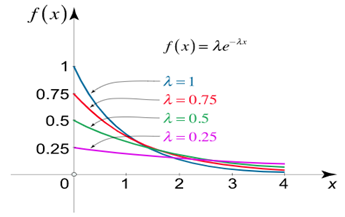
The mean value is μ = . The median of the exponential distribution is m = , and the variance is shown by .

Note-

If , then mean < Variance

If , then mean = Variance

If , then mean > Variance

The memoryless Property of Exponential Distribution

It can be stated as below

If X has an exponential distribution, then for every constant a 0, one has P[X x + a | X a] = P[X x] for all x i.e. the conditional probability of waiting up to the time 'x + a ' given that it exceeds ‘a’ is same as the probability of waiting up to the time ‘ x ’.

Key takeaways

1. A random variable X is said to follow the hypergeometric distribution with parameters N, M and n if it assumes only non-negative integer values and its probability mass function is given by

Where n, M, N are positive integers such that n ≤ N, M ≤ N.

2.     Mean of the Hyper-geometric distribution is given as-

3.     variance of hypergeometric dist is

4.     A random variable X is said to follow a continuous uniform distribution over an interval (a, b) if its probability density function is given by

5.     Mean and Variance of the continuous uniform Distribution

f(x)=λ,x≥0

Where, the rate λ signifies the

4.5 Normal distribution

The concept of normal distribution was given by English mathematician Abraham De Moivre in 1733 but the concrete theory was given by Karl Gauss that is why sometime normal distribution is called Gaussian distribution.

Normal distribution is a continuous distribution. It is derived a s the limiting form of the Binomial distribution for large values of n and p and q are not very small.

The Normal distribution is given by the equation

…. (1)

Where mean, standard deviation, , 

On substitution in (1), we get…. (2)

Here mean, standard deviation

(2) is known as standard form of normal distribution.

Graph of a normal probability function-

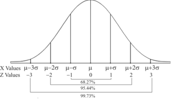
The curve looks like bell-shaped curve. The top of the bell is exactly above the mean.

If the value of standard deviation is large then curve tends to flatten out and for small standard deviation it has sharp peak.

This is one of the most important probability distributions in statistical analysis.

Mean for Normal Distribution:

Mean[Putting ]

Standard Deviation for Normal Distribution:

Put 

Median of the Normal Distribution

If a is the median, then it divides the total area into two equal halves so that,

Where

Suppose mean, then

[But]

(mean)

Thus

Similarly, when mean, we have

Thus, median=median.

Mean Deviation about the Mean

Mean Deviation

where

(As the function is given)

approximately.

Mode of the Normal distribution

We know that mode is the value of the variate x for which is maximum. Thus, by differential calculus is maximum if and

Where

Clearly will be maximum when the exponent will be maximum which will be the when

Thus, mode is and modal ordinate

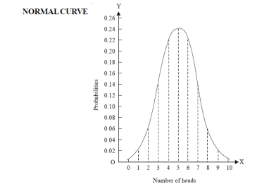
Let us show binomial distribution graphically. The probabilities of heads in 1 toss are.

. It is shown in the given figure.

If the variates (heads here) are treated as if they were continuous, the required probability curve will be a normal curve as shown in the above figure by dotted lines.

Properties of the normal curve:

1. The curve is symmetrical about the y – axis. The mean, median and mode coincide at the origin.
2. The curve is drawn, if mean (origin of x) and standard deviation are given. The value of can be calculated from the fact that the area of the curve must be equal to the total number of observations.
3. Y decreases rapidly as increases numericallu. The curve extends to infinity on either side of the origin.
4. (a)

(b)

(c) 

Hence (a) About of the values will lie between and .

(b) About 95% of the values will lie betweenand .

(c)  About 99.7% of the values will lie betweenand.

Area under the Normal curve

By taking , the standard normal curve is formed.

The total area under this curve is 1. The area under the curve is divided into two equal parts by. Left hand side are and right-hand side area to is . The area between the ordinate.

Example:

1. If X then find the probability density function of X.

2. If X then find the probability density function of X.

Sol.

1. We are given X

Here

We know that-

Then the p.d.f.  will be-

2. We are given X

Here

We know that-

Then the p.d.f.  will be-

Example. X is a normal variate with mean 30 and S.D. 5, find the probabilities that

(i)               

(ii)            

(iii)          |X-30|≥5

Solution. We have μ =30 and =5

(i)                When X = 26,z = -0.8, when X =40, z =-2

(ii)              When X =45, z =3

(iii)          

Example:

In a normal distribution 31% of the items are under 45 and 8% are over 64. Find the mean and standard deviation of the distribution.

Solution.

Let be the mean and the standard deviation 31% of the items are under 45 means area to the left of the ordinate x = 45

When x = 45, let z

From table III

When x = 64, let so that

Hence,

From table III

From (i) and (ii),

From (iii) and (iv),

Solving these equations we get

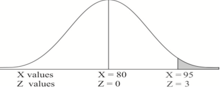
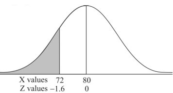
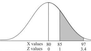
Example: If a random variable X is normally distributed with mean 80 and standard deviation 5, then find-

1. P[X > 95]

2. P[X < 72]

3. P [85 < X <97]

[Note- use the table- area under the normal curve]

Sol.

The standard normal variate is –

Now-

1. X = 95,

So that-

2. X = 72,

So that-

3. X = 85,

X = 97,

So that-

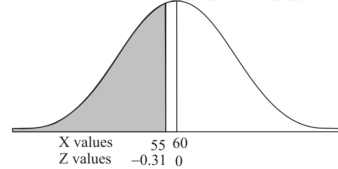
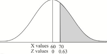
Example: In a company the mean weight of 1000 employees is 60kg and standard deviation is 16kg.

Find the number of employees having their weights-

1. Less than 55kg.

2. More than 70kg.

3. Between 45kg and 65kg.

Sol. Suppose X be a normal variate = the weight of employees.

Here mean 60kg and S.D. = 16kg

X

Then we know that-

We get from the data,

Now-

1. For X = 55,

So that-

2. For X = 70,

So that-

3. For X = 45,

For X = 65,

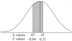
Hence the number of employees having weights between 45kg and 65kg-

Example: The mean inside diameter of a sample of 200 washers produced by a machine is 0.0502 cm and the standard deviation is 0.005 cm. The purpose for which these washers are intended allows a maximum tolerance in the diameter of 0.496 to 0.508 cm, otherwise the washers are considered defective. Determine the percentage of defective washers produced by the machine, assuming the diameters are normally distributed.

Sol.

Here-

And

Area for non-defective washers = area between z = -1.2 to +1.2

= 2 area between z = 0 and z = 1.2

= 2 × 0.3849 = 0.7698 = 76.98%

Then percent of defective washers = 100 – 76.98 = 23.02 %

Example: The life of electric bulbs is normally distributed with mean 8 months and standard deviation 2 months.

If 5000 electric bulbs are issued how many bulbs should be expected to need replacement after 12 months?

[Given that P (z ≥ 2) = 0. 0228]

Sol.

Here mean (μ) = 8 and standard deviation = 2

Number of bulbs = 5000

Total months (X) = 12

We know that-

Area (z ≥ 2) = 0.0228

Number of electric bulbs whose life is more than 12 months ( Z> 12)

= 5000 × 0.0228 = 114

Therefore, replacement after 12 months = 5000 – 114 = 4886 electric bulbs.

Key takeaways

1. The Normal distribution is given by the equation

Median=median.

2.     The curve is symmetrical about the y – axis. The mean, median and mode coincide at the origin.

3.     The curve is drawn, if mean (origin of x) and standard deviation are given. The value of can be calculated from the fact that the area of the curve must be equal to the total number of observations.

4.     Y decreases rapidly as increases numericallu. The curve extends to infinity on either side of the origin.

5.     a)

(b)

(c) 

4.6 Bivariate distributions

A bivariate distribution, set only, is the probability that a definite event will happen when there are 2 independent random variables in your scenario. E.g., having two bowls, individually complete with 2dissimilarkinds of candies, and drawing one candy from each bowl gives you 2 independent random variables, the 2dissimilar candies. Since you are pulling one candy from each bowl at the same time, you have a bivariate distribution when calculating your probability of finish up with specific types of candies.

Bivariate discrete random variables-

Let X and Y be two discrete random variables defined on the sample space S of a random experiment then the function (X, Y) defined on the same sample space is called a two-dimensional discrete random variable. In others words, (X, Y) is a two-dimensional random variable if the possible values of (X, Y) are finite or countably infinite. Here, each value of X and Y is represented as a point (x, y) in the xy-plane.

Joint probability mass function-

Let (X, Y) be two-dimensional discrete random variables with each possible outcome , we associate a number representing-

And satisfying the given conditions-

The function p defined for all is called joint probability mass function of X and Y.

Conditional probability mass function-

Let (X, Y) be a discrete two-dimensional random variable. Then the conditional probability mass function of X, given Y = y is defined as-

Because-

A bivariate distribution, set only, is the probability that a definite event will happen when there are 2 independent random variables in your scenario. E.g., having two bowls, individually complete with 2dissimilarkinds of candies, and drawing one candy from each bowl gives you 2 independent random variables, the 2dissimilar candies. Since you are pulling one candy from each bowl at the same time, you have a bivariate distribution when calculating your probability of finish up with specific types of candies.

Properties:

Property-1

Two random variables X and Y are said to be bivariate normal, or jointly normal distribution for all

Properties 2:

Two random variables X and Y are set to have the standard bivariate normal distribution with correlation efficient if their joint PDF is given by

Where then we just say X and Y have the standard by will it normal distribution.

Properties 3:

Two random variables X and Y are set to have a bivariate normal distribution with parameters if their joint PDF is given by

Where are all constants.

Properties 4:

Suppose X and Y are jointly normal random variables with parameters . Then given X = x, Y is normally distributed with

Example.

Let be two independent N (0, 1) random variables. Define

Where is a real number in (-1, 1)

1. Show that X and Y are bivariate normal.
2. Find the joint PDF of X and Y.
3. Find (X, Y)

Solution.

First note that since are normal and independent they are jointly normal with the joint PDF

1. We need to show aX + bY is normal for all. We have

Which is the linear combination of and thus it is normal.

b.     We can use the method of transformations (theorem 5.1) to find the joint PDF of X and Y. The inverse transformation is given by

We have

Where,

Thus, we conclude that

c.      To find FIRST NOTE

Therefore,

Example:

Let X and Y be jointly normal random variable with parameters

1. Find P (2X+ Y≤3)
2. Find
3. Find

Solution.

1. Since X and Y are jointly normal the random variables V =2 X +Y is normal. We have

Thus V ~ N (2, 12). Therefore,

b.     Note that Cov (X, Y)= (X,Y) =1. We have

c.      Using properties, we conclude that given X =2, Y is normally distributed with

Example:

Let X and Y be jointly normal random variables with parameters Find the conditional distribution of Y given X =x.

Sol. One way to solve this problem is by using the joint PDF formula since X N we can use

Thus given X=x, we have

And,

Since are independent, knowing does not provide any information on . We have shown that given X=x, Y is a linear function of , thus it is normal. Ln particular

We conclude that given X=x, Y is normally distributed with mean and variance
 

Key takeaways-

References:

1. E. Kreyszig, “Advanced Engineering Mathematics”, John Wiley & Sons, 2006.
2. P. G. Hoel, S. C. Port and C. J. Stone, “Introduction to Probability Theory”, Universal Book Stall, 2003.
3. S. Ross, “A First Course in Probability”, Pearson Education India, 2002.
4. W. Feller, “An Introduction to Probability Theory and Its Applications”, Vol. 1, Wiley, 1968.
5. N.P. Bali and M. Goyal, “A Text Book of Engineering Mathematics”, Laxmi Publications, 2010.
6. B.S. Grewal, “Higher Engineering Mathematics”, Khanna Publishers, 2000.
7. T. Veerarajan, “Engineering Mathematics”, Tata McGraw-Hill, New Delhi, 2010
8. Higher engineering mathematics, HK Dass
9. IGNOU
10. Fundamentals of mathematical statistics by SC Gupta and VK kapoor