Module-4

Vector integral calculus

4.1 Line Integrals

The Line Integral

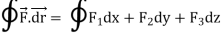
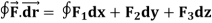
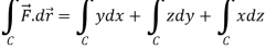
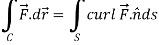
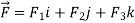
Let- F be vector function defined throughout some region of space and let C be any curve in that region. ṝ is the position vector of a point p (x,y,z) on C then the integral ƪ F .dṝ is called the line integral of  F taken over

Now, since ṝ =xi+yi+zk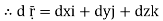

And if F͞ =F1i + F2 j+ F3  K

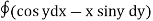
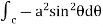
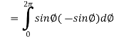
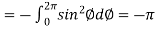
Q1. Evaluate where F= cos y.i-x siny j and C is the curve y= in the xy plae from (1,0) to (0,1)

Solution: The curve y= i.e x2+y2 =1. Is a circle with centre at the origin and radius unity.

=

=

=       =-1

Q2. Evaluate where = (2xy +z2) I +x2j +3xz2 k along the curve x=t, y=t2, z= t3 from (0,0,0) to (1,1,1).

 Solution:    F x dr =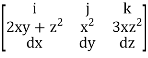

 Put x=t, y=t2, z= t3

Dx=dt ,dy=2tdt,                dz=3t2dt.

F x dr =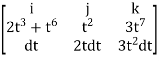

=(3t4-6t8) dti  – ( 6t5+3t8 -3t7) dt j +( 4t4+2t7-t2)dt k

=t4-6t3)dti –(6t5+3t8-3t7)dt j+(4t4 + 2t7 – t2)dt k

=

=+

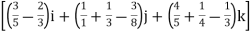
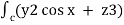
Example 3: Prove that   ͞͞͞F = [y2cos x +z3] i+(2y sin x – 4) j +(3xz2 + 2) k is a conservative field. Find (i) scalar potential for͞͞͞F  (ii) the work done in moving an object in this field from (0, 1, -1) to (/ 2,-1, 2)

Sol.: (a) The field is conservative if cur͞͞͞͞͞͞F = 0.

Now, curl͞͞͞ F = ̷̷ X                    / y            / z

                            Y2COS X +Z3        2y sin x-4     3xz2 + 2

; Cur = (0-0) – (3z2 – 3z2) j + (2y cos x- 2y cos x) k = 0

; F is conservative.

(b) Since F is conservative there exists a scalar potential ȸ such that

F = ȸ

(y2cos x=z3) i + (2y sin x-4) j + (3xz2 + 2) k =   i +   j + k

= y2cos x + z3, = 2y sin x – 4, = 3xz2 + 2

Now, = dx + dy + dz

= (y2cos x + z3) dx +(2y sin x – 4)dy + (3xz2 + 2)dz

= (y2cos x dx + 2y sin x dy) +(z3dx +3xz2dz) +(- 4 dy) + (2 dz)

=d(y2 sin x + z3x – 4y -2z)

ȸ = y2 sin x +z3x – 4y -2z

(c)  now, work done = .d   ͞r

=  dx + (2y sin x – 4) dy + ( 3xz2 + 2) dz

=   (y2 sin x + z3x – 4y + 2z)    (as shown above)

= [ y2 sin x + z3x – 4y + 2z ]( /2, -1, 2)

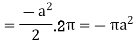
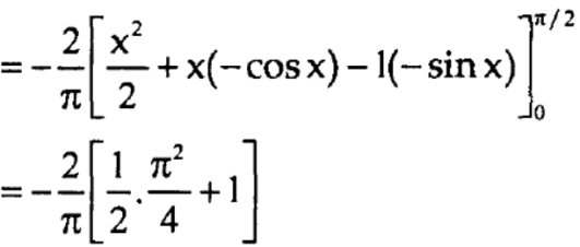
= [ 1 +8 + 4 + 4 ] – { - 4 – 2} =4 + 15

Sums Based on Line Integral

1. Evaluate where =yz i+zx  j+xy k and C is the position of the curve.

= (a cost)i+(b sint)j+ct k , from y=0 to t=π/4.

Sol.:  = (a cost)i+(b sint)j+ct k

 The parametric eqn. of the curve are x= a cost, y=b sint, z=ct              (i)

=

 Putting values of x,y,z from (i),

dx=-a sint

dy=b cost

dz=c dt

=

=

==

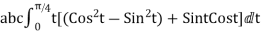
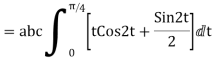
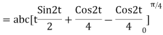
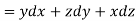
2. Find the circulation of around the curve C where =yi+zj+xk and C is circle .

Soln. Parametric eqn of circle are:

x=a cos

y=a sin

z=0

=xi+yj+zk = a cosi + b cos + 0 k

d=(-a sin i + a cos j)d

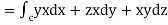
Circulation = =+zj+xk). d

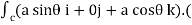=-a sin i + a cos j)d

= =

Key takeaways-

When the path of integration is closed curve then we use the notation for integration-

  in place of

4.2 Green Theorem

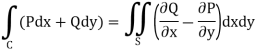
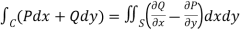
Green’s theorem in a plane

If C be a regular closed curve in the xy-plane and S is the region bounded by C then,

Where P and Q are the continuously differentiable functions inside and on C.

Green’s theorem in vector form-

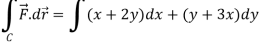
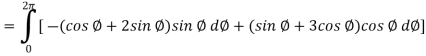
Example-1: Apply Green’s theorem to evaluate where C is the boundary of the area enclosed by the x-axis and the upper half of circle

Sol. We know that by Green’s theorem-

And it it given that-

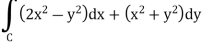
Now comparing the given integral-

P =   and   Q =

Now-

and

So that by Green’s theorem, we have the following integral-

Example-2: Evaluate by using Green’s theorem, where C is a triangle formed by

Sol. First we will draw the figure-

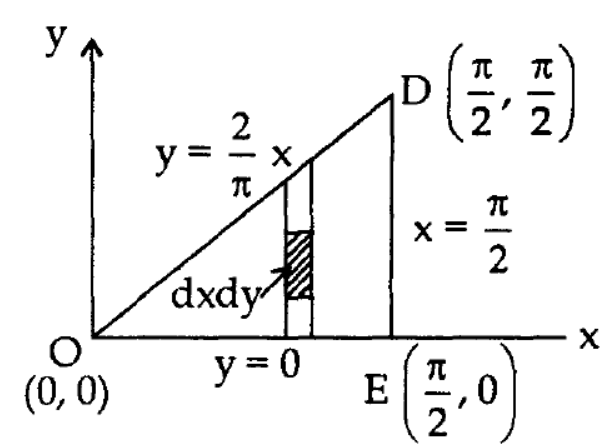
Here the vertices of triangle OED are (0,0), (

Now by using Green’s theorem-

Here P = y – sinx, and Q  =cosx

So that-

and

Now-

=

Which is the required answer.

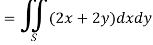
Example-3: Verify green’s theorem in xy-plane for 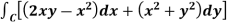where C is the boundary of the region enclosed by

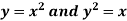
Sol.

On comparing with green’s theorem,

We get-

P = and Q =

and

By using Green’s theorem-

  ………….. (1)

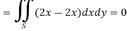
And left hand side=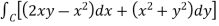

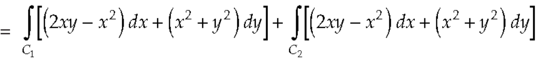………….. (2)

Now,

Along

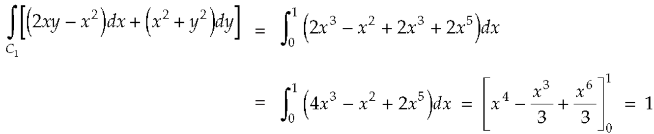
Along

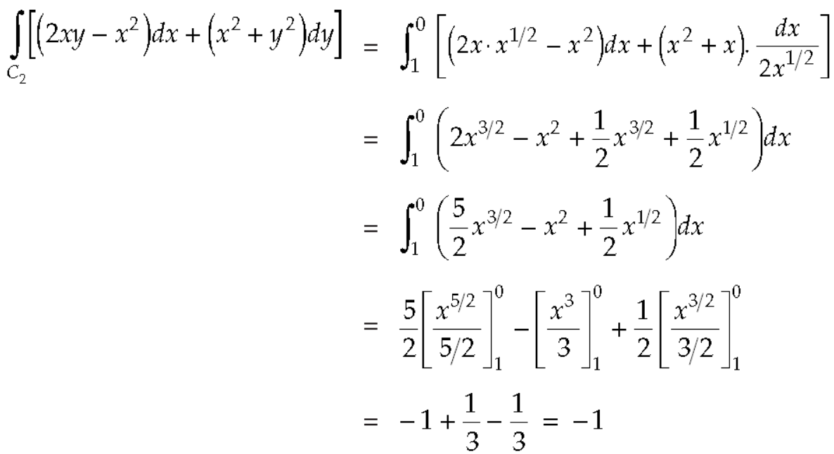
Put these values in (2), we get-

               L.H.S. = 1 – 1 = 0

So that the Green’s theorem is verified.

4.3 Surface integrals

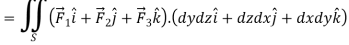
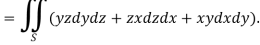
Surface integrals-

An integral which we evaluate over a surface is called a surface integral.

                   Surface integral =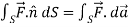

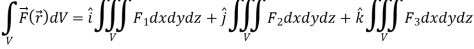
Volume integrals-

The volume integral is denoted by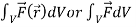

And defined as-

If  , then

Note-

If in a conservative field 

Then this is the condition for independence of path.

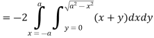
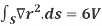
Example: Evaluate 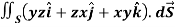, where S is the surface of the sphere in the first octant.

Sol. Here-

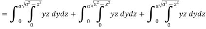
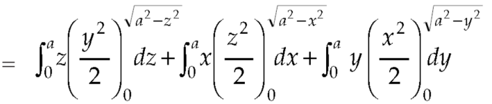
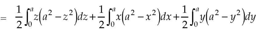
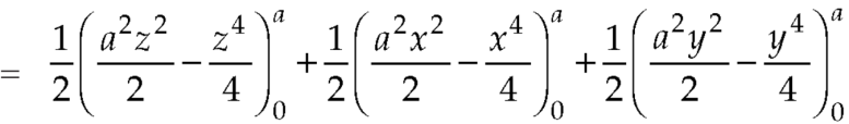
Which becomes-

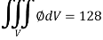
Example: Evaluate , where and V is the closed reason bounded by the planes 4x + 2y + z = 8, x = 0, y = 0, z = 0.

Sol.

Here-   4x + 2y + z = 8

Put y = 0 and z = 0 in this, we get

4x = 8 or x = 2

Limit of x varies from 0 to 2 and y varies from 0 to 4 – 2x

And z varies from 0 to 8 – 4x – 2y

So that-

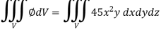
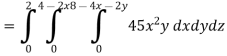
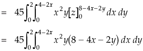
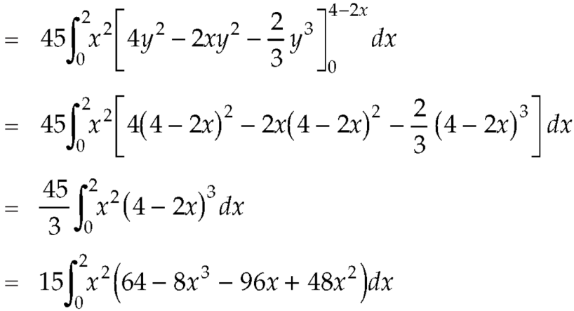
So that-

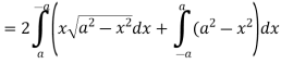
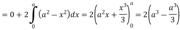
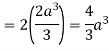
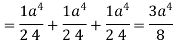
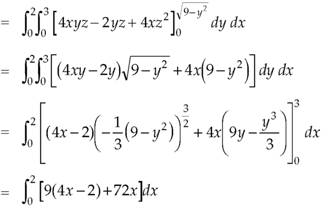
Example: Evaluate if V is the region in the first octant bounded by and the plane x = 2 and .

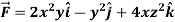Sol.

x varies from 0 to 2

The volume will be-

Key takeaways-

Surface integral =

The volume integral is denoted by

3.     If in a conservative field 

Then this is the condition for independence of path

4.4 Gauss theorem and Stokes Theorem (Without Proof)

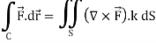
Stoke’s theorem (without proofs) and their verification-

If is any continuously differentiable vector point function and S is a surface bounded by a curve C, then-

Example-1: Verify stoke’s theorem when and surface S is the part of sphere , above the xy-plane.

Sol.

We know that by stoke’s theorem,

Here C is the unit circle-

So that-

Now again on the unit circle C, z = 0

dz = 0

Suppose, 

And           

Now

  ……………… (1)

Now-

Curl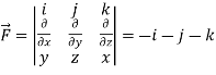

Using spherical polar coordinates-

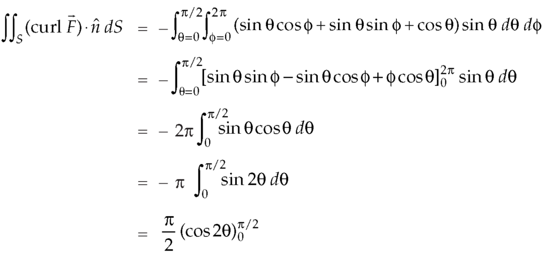
  ………………… (2)

From equation (1) and (2), stoke’s theorem is verified.

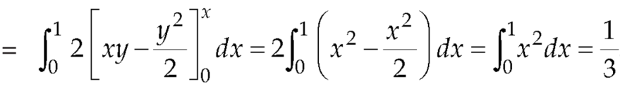
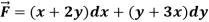
Example-2: If 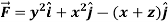and C is the boundary of the triangle with vertices at (0, 0, 0), (1, 0, 0) and (1, 1, 0), then evaluate by using Stoke’s theorem.

Sol. here we see that z-coordinates of each vertex of the triangle is zero, so that the triangle lies in the xy-plane and

Now,

Curl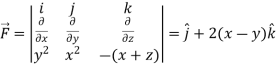

Curl

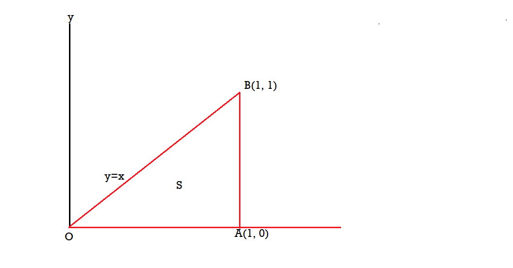
The equation of the line OB is y = x

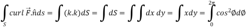
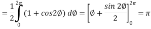
Now by stoke’s theorem,

Example-3: Verify Stoke’s theorem for the given function-

Where C is the unit circle in the xy-plane.

Sol. Suppose-

Here

We know that unit circle in xy-plane-

Or

So that,

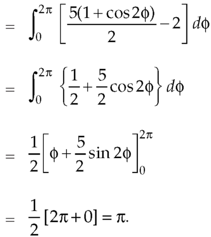
Now

Curl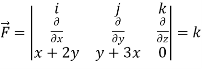

Now,

Hence the Stoke’s theorem is verified.

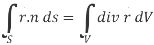
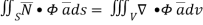
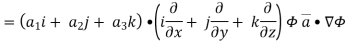
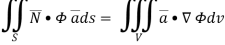
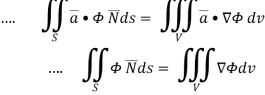
Gauss divergence theorem

If V is the volume bounded by a closed surface S and is a vector point function with continuous derivative-

Then it can be written as-

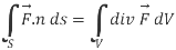
where unit vector to the surface S.

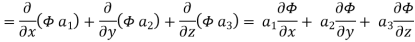
Example-1: Prove the following by using Gauss divergence theorem-

1.

2.

Where S is any closed surface having volume V and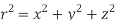

Sol. Here we have by Gauss divergence theorem-

Where V is the volume enclose by the surface S.

We know that-

= 3V

2.

Because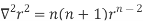 

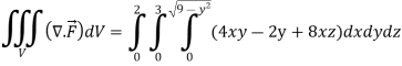
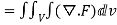
Example – 2 Show that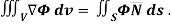 

Sol

By divergence theorem,  ..…(1)

Comparing  this  with  the  given  problem  let 

Hence, by (1)

                                    ………….(2)

Now ,

Hence, from (2), We get,

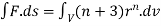
Example Based on Gauss Divergence Theorem

Show that

Soln.  We have Gauss Divergence Theorem

 By data, F=  

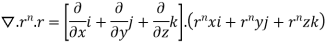
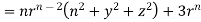
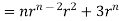
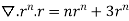
=(n+3)

2 Prove that  =

Soln. By Gauss Divergence Theorem,

=

= =

.[

=

References