Unit-1
Introduction
Basically algorithms are the finite steps to solve problems in computers.
It can be the set of instructions that performs a certain task.
The collection of unambiguous instructions occurring in some specific sequence and such a procedure should produce output for a given set of input in a finite amount of time is known as Algorithm.
Algorithms are defined to be a step by step method to solve certain problems. For example if you need to write a program to calculate the age of a person let us say after 5 years so in programming we need to take some input, process it and then provide an output.
Algorithm for the above scenario will be the steps used in order to calculate age after 5 years.
A simple algorithm for this scenario can be written as follow: -
Step 1: - Take the input as the current age of the person.
Step 2: - Perform the calculation i.e. add 5 years to his current age
Step 3: - Output will be a value obtained after calculation which is his age after 5 years.
An algorithm to be any well-defined computational procedure that takes some values as input and produces some values as output.
An algorithm is a finite set of instructions that, if followed, accomplishes a particular task. An algorithm is a sequence of unambiguous instructions for solving a problem, i.e., for obtaining a required output for any legitimate input in a finite amount of time.
Characteristics of algorithm
There are five main characteristics of an algorithm which are as follow:-
● Input: - Any given algorithm must contain an input the format of the input may differ from one another based on the type of application, certain application needs a single input while others may need “n” inputs at initial state or might be in the intermediate state.
● Output: - Every algorithm which takes the input leads to certain output. An application for which the algorithm is written may give output after the complete execution of the program or some of them may give output at every step.
● Finiteness: - Every algorithm must have a proper end, this proper end may come after certain no of steps. Finiteness here can be in terms of the steps used in the algorithm or it can be in the term of input and output size (which should be finite every time).
● Definiteness: - Every algorithm should define certain boundaries, which means that the steps in the algorithm must be defined precisely or clearly.
● Effectiveness: - Every algorithm should be able to provide a solution which successfully solves that problem for which it is designed.
Analysis of the algorithm is the concept of checking the feasibility and optimality of the given algorithm, an algorithm is feasible and optimal if it is able to minimize the space and the time required to solve the given problem.
Key takeaway:
In the theoretical study of algorithms, it is usual to estimate the complexity function in an asymptotic sense, that is, for arbitrarily large input. Donald Knuth developed the phrase "analysis of algorithms."
The study of algorithms is an essential component of computational complexity theory. It calculates the needed resources for an algorithm to solve a certain computing issue theoretically. The majority of algorithms are made to function with inputs of any length. The assessment of the amount of time and space resources necessary to execute an algorithm is known as algorithm analysis.
Typically, an algorithm's efficiency or running time is expressed as a function linking the input length to the number of steps (time complexity) or the amount of memory (space complexity).
The Importance of Research
In this chapter, we'll talk about why it's important to analyse algorithms and how to pick the best algorithm for a given issue, because one computing issue can be handled by a variety of algorithms.
By analysing an algorithm for a specific problem, we may begin to create pattern recognition, allowing this algorithm to tackle similar sorts of issues.
Algorithms are frequently fairly distinct from one another, despite the fact that their goals are the same. We know, for example, that a collection of integers may be sorted using several techniques. For the same input, the number of comparisons conducted by one algorithm may differ from that of others. As a result, the temporal complexity of such methods may vary. At the same time, we must determine how much RAM each method requires.
The process of examining the algorithm's problem-solving abilities in terms of the time and size required is known as algorithm analysis (the size of memory for storage while implementation). However, the most important consideration in algorithm analysis is the needed time or performance.
In general, we do the following sorts of research:
To solve an issue, we must consider both time and space complexity, since the software may execute on a device with limited memory but plenty of space, or vice versa. If we compare bubble sort with merge sort in this scenario. Bubble sorting does not need more memory, but merge sorting does. Though bubble sort has a greater time complexity than merge sort, it may be necessary to use it if the application must execute in a memory-constrained environment.
Following are the conditions where we can analyse the algorithm:
● Time efficiency:- indicates how fast algorithm is running
● Space efficiency:- how much extra memory the algorithm needs to complete its execution
● Simplicity: - generating sequences of instruction which are easy to understand.
● Generality: - It fixes the range of inputs it can accept. The generality of problems which algorithms can solve.
It is a formal way to speak about functions and classify them.
It is used to specify the running time and space complexity of an algorithm and to frame the run time performance in mathematical computation.
It refers to boundation or framing into the mathematical terms.
As the algorithm has three cases according to time taken by program to perform a certain task.
Following are the asymptotic notations which are used to calculate the running time complexity of algorithm:
Big Oh (O) Notation :
● It is the formal way to express the time complexity.
● It is used to define the upper bound of an algorithm’s running time.
● It shows the worst case time complexity or largest amount of time taken by the algorithm to perform a certain task.
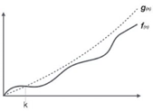
Fig 1: Big Oh notation
Here, f( n ) <= g( n ) ……………..(eq1)
where n>= k , C>0 and k>=1
if any algorithm satisfies the eq1 condition then it becomes f ( n )= O ( g ( n ) )
Big Omega (ῼ) Notation
● It is the formal way to express the time complexity.
● It is used to define the lower bound of an algorithm’s running time.
● It shows the best case time complexity or best of time taken by the algorithm to perform a certain task.

Fig 2: Big omega notation
Here, f ( n ) >= g ( n )
where n>=k and c>0, k>=1
if any algorithm satisfies the eq1 condition then it becomes f ( n )= ῼ ( g ( n ) )
Theta (Θ) Notation
● It is the formal way to express the time complexity.
● It is used to define the lower as well as upper bound of an algorithm’s running time.
● It shows the average case time complexity or average of time taken by the algorithm to perform a certain task.

Fig 3: Theta notation
Let C1 g(n) be upper bound and C2 g(n) be lower bound.
C1 g(n)<= f( n )<=C2 g(n)
Where C1, C2>0 and n>=k
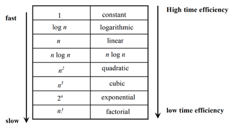
Basic Efficiency classes
The time efficiencies of a large number of algorithms fall into only a few classes
Key takeaway:
The general framework for analyzing the efficiency of algorithms could be the time and space efficiency.
Time efficiency indicates how fast an algorithm in question runs. Space efficiency deals with the extra space the algorithm requires.
Unit for measuring running time would be of primary consideration when estimating an algorithm’s performance is the number of basic operations required by the algorithm to process an input of a certain size.
The terms “basic operations” and “size” are both rather vague and depend on the algorithm being analysed. Size is often the number of inputs processed.
For example, when comparing sorting algorithms, the size of the problem is typically measured by the number of records to be sorted. A basic operation must have the property that it’s time to complete does not depend on the particular values of its operands.
Adding or comparing two integer variables are examples of basic operations in most programming languages. Summing the contents of an array containing n integers is not, because the cost depends on the value of n (i.e., the size of the input).
Example: Consider a simple algorithm to solve the problem of finding the largest value in an array of n integers. The algorithm looks at each integer in turn, saving the position of the largest value seen so far. This algorithm is called the largest-value sequential search and is illustrated by the following Java function:
// Return position of largest value in "A"
static int largest (int [] A) {
int curlarge = 0; // Holds largest element position
for (int i=1; i<A.length; i++) // For each element
if (A[curlarge] < A[i]) // if A[i] is larger
curlarge = i; // remember its position
return curlarge; // Return largest position
}
Here, the size of the problem is n, the number of integers stored in A.
The basic operation is to compare an integer’s value to that of the largest value 60. It is reasonable to assume that it takes a fixed amount of time to do one such comparison, regardless of the value of the two integers or their positions in the array.
As the most important factor affecting running time is normally size of the input, for a given input size n we often express the time T to run the algorithm as a function of n, written as T(n). We will always assume T(n) is a non-negative value.
Let us call c the amount of time required to compare two integers in function largest. We do not care right now what the precise value of c might be. Nor are we concerned with the time required to increment variable i because this must be done for each value in the array, or the time for the actual assignment when a larger value is found, or the little bit of extra time taken to initialize curlarge.
We just want a reasonable approximation for the time taken to execute the algorithm. The total time to run largest is therefore approximately cn, because we must make n comparisons, with each comparison costing c time.
We say that function largest (and the largest-value sequential search algorithm in general) has a running time expressed by the equation
T(n) = cn.
This equation describes the growth rate for the running time of the largest value sequential search algorithm.
The growth rate for an algorithm is the rate at which the cost of the algorithm grows as the size of its input grows. Figure shows a graph for six equations, each meant to describe the running time for a particular program or algorithm.
A variety of growth rates representative of typical algorithms are shown. The two equations labeled 10n and 20n are graphed by straight lines. A growth rate of cn (for c any positive constant) is often referred to as a linear growth rate or running time.
This means that as the value of n grows, the running time of the algorithm grows in the same proportion. Doubling the value of n roughly doubles the running time. An algorithm whose running- time equation has a highest-order term containing a factor of n2 is said to have a quadratic growth rate.
In Figure, the line labeled 2n2 represents a quadratic growth rate. The line labeled 2n represents an exponential growth rate. This name comes from the fact that n appears in the exponent. The line labeled n! is also growing exponentially.
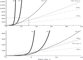
Fig 4: Two views of a graph illustrating the growth rates for six equations.
The bottom view shows in detail the lower-left portion of the top view. The horizontal axis represents input size. The vertical axis can represent time, space, or any other measure of cost.
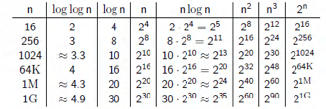
Fig 5: Costs for growth rates representative of most computer algorithms.
Both time and space efficiencies are measured as functions of the algorithm's input size.
Time efficiency is measured by counting the no. of times the algorithm’s basic operation is executed. Space efficiency is measured by counting the number of extra memory units consumed by the algorithm.
The efficiencies of some algorithms may differ significantly for inputs of the same size. For such algorithms, one has to distinguish between the worst case, average case and best case efficiencies.
The framework’s primary interest lies in the order of growth of the algorithm’s running time as its input size goes to infinity.
Key takeaway :
● It is also known as time memory trade off.
● It is a way of solving problems in less time by using more storage space.
● It can be used with the problem of data storage.
● For example: time complexity of merge sort is O(n log n)in all cases. But requires an auxiliary array.
● In quick sort complexity is O(n log n) for best and average case but it doesn’t require auxiliary space.
● Two Space-for-Time Algorithm Varieties:
● Input enhancement - To store some info, preprocess the input (or its portion) to be used in solving the issue later
● counting sorts
● string searching algorithms
● Pre-structuring-pre-processing the input to access its components
Key takeaway :
A recurrence is an equation or inequality that on smaller inputs describes a function in terms of its values. Solving a recurrence relationship means obtaining a function that is defined by the natural numbers that satisfy the recurrence.
For instance, the recurrence describes the worst case running time T(n) of the MERGE SORT Procedures.
T (n) = θ (1) if n=1
2T + θ (n) if n>1
For solving recurrence, there are four methods:
Substitution Method
There are two main steps in the Substitution Method:
Example : The Substitution Method solves the equation.
T (n) = T + n
+ n
We have to demonstrate that it is bound asymptotically by O (log n).
Solution :
For T (n) = O (log n)
We must show that for some constant c, for some constant c,
T (n) ≤c log n.
Place this in the Recurrence Equation given.
T (n) ≤c log + 1
+ 1
≤c log + 1 = c logn-clog2 2+1
≤c log n for c≥1
Thus T (n) =O log n.
Key takeaway :
● The Recursion Tree Method is a pictorial representation of a method of iteration in the form of a tree where nodes are expanded at each level.
● In particular, in recurrence, we consider the second term as the root.
● When the divide & Conquer algorithm is used, it is useful.
● A good guess is sometimes hard to come up with. Each root and child in the Recursion tree represents the cost of a single sub-problem.
● In order to obtain a set of pre-level costs, we sum up the costs within each of the tree levels and then sum up all pre-level costs to determine the total cost of all recursion levels.
● To generate a good guess, which can be verified by the Substitution Method, a Recursion Tree is best used.
Example : Consider the recurrence of the following
T (n) = 4T +n
+n
Using the recursion tree method to obtain the asymptotic bond.
Solution : For the above mentioned recurrence, the recursion trees
|
Fig 6: Recursion tree

Master’s Theorem
To solve the following recurrence forms, the Master Method is used
T (n) = a T + f (n) with a≥1 and b≥1 be constant & f(n) be a function and
  can be interpreted as
On non-negative integers, let T(n) be determined by the recurrence.
T (n) = a T + f (n)
The constants and functions take on the following sense in the function for the study of a recursive algorithm:
● n reflects the size of the problem.
● a is the number of recursion sub-problems.
● The size of each sub-problem is n/b. (All sub-problems are considered to be approximately the same size here.)
● F(n) is the sum of the work performed beyond the recursive calls, namely the sum of the problem division and the sum of the solutions to the subproblems combined.
● The function can not always be bound according to the requirement, so we make three instances that will tell us what sort of bound we can apply to the function.
Master Theorem
In these three cases, it is possible to complete an asymptotic strong bound:
Case1: If f (n) =  for some constant ε >0, then it follows that:
T (n) = Θ 
Case2 : If it is real, this is: for any constant k ≥ 0
F (n) = Θ  then it follows that: T (n) = Θ
Case3: If it is true f(n) = Ω  for some constant ε >0 and it also true that : a f
  for some constant c<1 for large value of n ,then :
T (n) = Θ((f (n))
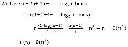
Example :
Solve the relationship with recurrence:
T (n) = 2 
Solution :
Compare the given issue with the problem, T (n) = a T

a= 2, b =2, f (n) = n2, logba = log22 =1
Put in all values f (n) = Ω  ..... (Eq. 1)
If we enter all of the value in (Eq.1), we will obtain
n2 = Ω(n1+ε) put ε =1, Then equality can be maintained.
n2 = Ω(n1+1) = Ω(n2)
Now we'll verify the second condition as well:
2 
If we choose c = 1/2, the truth is:
 ∀ n ≥1
So it follows: T (n) = Θ ((f (n))
T (n) = Θ(n2)
Key takeaway :
References:
1. Introduction to Algorithms, 4TH Edition, Thomas H Cormen, Charles E Lieserson, Ronald L Rivest and Clifford Stein, MIT Press/McGraw-Hill.
2. Fundamentals of Algorithms – E. Horowitz et al.
3. Design and Analysis of Algorithms, M.R.Kabat, PHI Learning
4. Algorithm Design, 1ST Edition, Jon Kleinberg and ÉvaTardos, Pearson.
5. Algorithm Design: Foundations, Analysis, and Internet Examples, Second Edition, Michael T Goodrich and Roberto Tamassia, Wiley.
6. Algorithms—A Creative Approach, 3RD Edition, UdiManber, Addison-Wesley,
Reading, MA.
