Unit - 2
Fundamental Algorithmic Strategies
Algorithm:
An algorithm is a step-by-step procedure to solve a problem. A good algorithm should be optimized in terms of time and space. Different types of problems require different types of algorithmic-techniques to be solved in the most optimized manner. There are many types of algorithms but the most important and the fundamental algorithms that you must know will be discussed in this article.
Brute Force Algorithm:
This is the most basic and simplest type of algorithm. A Brute Force Algorithm is the straightforward approach to a problem i.e., the first approach that comes to our mind on seeing the problem. More technically it is just like iterating every possibility available to solve that problem.
For Example: If there is a lock of 4-digit PIN. The digits to be chosen from 0-9 then the brute force will be trying all possible combinations one by one like 0001, 0002, 0003, 0004, and so on until we get the right PIN. In the worst case, it will take 10,000 tries to find the right combination.
Recursive Algorithm:
This type of algorithm is based on recursion. In recursion, a problem is solved by breaking it into subproblems of the same type and calling own self again and again until the problem is solved with the help of a base condition.
Some common problem that is solved using recursive algorithms are Factorial of a Number, Fibonacci Series, Tower of Hanoi, DFS for Graph, etc.
Divide and Conquer Algorithm:
In Divide and Conquer algorithms, the idea is to solve the problem in two sections, the first section divides the problem into subproblems of the same type. The second section is to solve the smaller problem independently and then add the combined result to produce the final answer to the problem.
Some common problem that is solved using Divide and Conquers Algorithms are Binary Search, Merge Sort, Quick Sort, Strassen’s Matrix Multiplication, etc.
Dynamic Programming Algorithms:
This type of algorithm is also known as the memorization technique because in this the idea is to store the previously calculated result to avoid calculating it again and again. In Dynamic Programming, divide the complex problem into smaller overlapping sub problems and storing the result for future use.
The following problems can be solved using Dynamic Programming algorithm Knapsack Problem, Weighted Job Scheduling, Floyd Warshall Algorithm, Dijkstra Shortest Path Algorithm, etc.
Greedy Algorithm:
In the Greedy Algorithm, the solution is built part by part. The decision to choose the next part is done on the basis that it gives the immediate benefit. It never considers the choices that had taken previously.
Some common problems that can be solved through the Greedy Algorithm are Prim’s Algorithm, Kruskal’s Algorithm, Huffman Coding, etc.
Backtracking Algorithm:
In Backtracking Algorithm, the problem is solved in an incremental way i.e., it is an algorithmic-technique for solving problems recursively by trying to build a solution incrementally, one piece at a time, removing those solutions that fail to satisfy the constraints of the problem at any point of time.
Brute Force Attack
A Brute force attack is a well-known breaking technique, by certain records, brute force attacks represented five percent of affirmed security ruptures. A brute force attack includes ‘speculating’ username and passwords to increase unapproved access to a framework. Brute force is a straightforward attack strategy and has a high achievement rate.
A few attackers use applications and contents as brute force devices. These instruments evaluate various secret word mixes to sidestep confirmation forms. In different cases, attackers attempt to get to web applications via scanning for the correct session ID. Attacker inspiration may incorporate taking data, contaminating destinations with malware, or disturbing help.
While a few attackers still perform brute force attacks physically, today practically all brute force attacks are performed by bots. Attackers have arrangements of usually utilized accreditations, or genuine client qualifications, got through security breaks or the dull web. Bots deliberately attack sites and attempt these arrangements of accreditations, and advise the attacker when they obtain entrance.
Types of Brute Force Attacks:
How to Prevent Brute Force Password Hacking?
To protect your organization from brute force password hacking, enforce the use of strong passwords.
Passwords should:
Key takeaways:
Brute Force Algorithm:
This is the most basic and simplest type of algorithm. A Brute Force Algorithm is the straightforward approach to a problem i.e., the first approach that comes to our mind on seeing the problem. More technically it is just like iterating every possibility available to solve that problem.
For Example: If there is a lock of 4-digit PIN. The digits to be chosen from 0-9 then the brute force will be trying all possible combinations one by one like 0001, 0002, 0003, 0004, and so on until we get the right PIN. In the worst case, it will take 10,000 tries to find the right combination.
Linear search
Linear search, also known as sequential search, is the most basic search algorithm. In this method of quest, we basically go through the whole list and match each element to the object whose location needs to be identified. If a match is made, the algorithm returns the item's location; otherwise, NULL is returned.
Linear search is most often used to find elements in an unordered array that aren't sorted. The above is the linear search algorithm.
Problem:
Given an array arr [] of n elements, write a function to search a given element x in arr [].
Examples:
Input: arr [] = {10, 20, 80, 30, 60, 50,
110, 100, 130, 170}
x = 110;
Output: 6
Element x is present at index 6
Input: arr [] = {10, 20, 80, 30, 60, 50,
110, 100, 130, 170}
x = 175;
Output: -1
Element x is not present in arr [].
A straightforward method is to do a linear search, i.e.
Begin with arr [leftmost]'s part. and compare x with each element of arr [] one by one
Return the index if x matches an element.
Return -1 if x does not fit any of the elements.
Selection sort
In selection type, the smallest value among the array's unsorted elements is chosen in each pass and put into the appropriate location.
To begin, locate the array's smallest element and place it in the first location. Then locate the array's second smallest member and put it in the second location. The procedure is repeated before the sorted list is obtained.
The array with n elements is sorted by using n-1 pass of selection sort algorithm.
The smallest member of the array, as well as its index pos, must be located in the first pass. Swap A [0] and A[pos] after that. As a result of sorting A [0], we now have n -1 elements to handle.
The place pos of the smallest element in the sub-array A[n-1] is located in the second pas. Swap A [1] and A[pos] after that. After sorting A [0] and A [1], we're left with n-2 unsorted items.
The place pos of the smaller element between A[n-1] and A[n-2] must be located in the n-1st move. Swap A[pos] and A[n-1] after that.
As a result, the elements A [0], A [1], A [2] ...., A[n-1] are sorted using the method described above.
SELECTION SORT (ARR, N)
[END OF LOOP]
Greedy
In optimization problems, a greedy algorithm is a simple, intuitive algorithm. As it tries to find the ultimate best solution to the problem, the algorithm takes the best decision at each stage. Some greedy algorithms, such as Huffman encoding, which is used to compress data, and Dijkstra's algorithm, which is used to find the shortest path between two points, are very efficient.
However, in many cases, a greedy approach does not yield the best result. The greedy algorithm, for example, searches out the course with the highest amount in the animation below. It accomplishes this by choosing the maximum number available at each level.
The greedy algorithm, on the other hand, struggles to find the largest number because it takes decisions based solely on the knowledge available at any given time, with little respect for the larger dilemma.
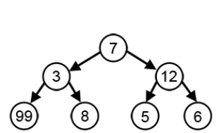
Fig 2.1 Greedy Algorithm
(i) Data can be encoded efficiently using Huffman Codes.
(ii) It is a widely used and beneficial technique for compressing data.
(iii) Huffman's greedy algorithm uses a table of the frequencies of occurrences of each character to build up an optimal way of representing each character as a binary string.
Suppose we have 105 characters in a data file. Normal Storage: 8 bits per character (ASCII) - 8 x 105 bits in a file. But we want to compress the file and save it compactly. Suppose only six characters appear in the file:

How can we represent the data in a Compact way?
(i) Fixed length Code: Each letter represented by an equal number of bits. With a fixed length code, at least 3 bits per character:
For example:
a 000
b 001
c 010
d 011
e 100
f 101
For a file with 105 characters, we need 3 x 105 bits.
(ii) A variable-length code: It can do considerably better than a fixed-length code, by giving many characters short code words and infrequent character long codewords.
For example:
a 0
b 101
c 100
d 111
e 1101
f 1100
Number of bits = (45 x 1 + 13 x 3 + 12 x 3 + 16 x 3 + 9 x 4 + 5 x 4) x 1000
= 2.24 x 105bits
Thus, 224,000 bits to represent the file, a saving of approximately 25%. This is an optimal character code for this file.
The prefixes of an encoding of one character must not be equal to complete encoding of another character, e.g., 1100 and 11001 are not valid codes because 1100 is a prefix of some other code word is called prefix codes.
Prefix codes are desirable because they clarify encoding and decoding. Encoding is always simple for any binary character code; we concatenate the code words describing each character of the file. Decoding is also quite comfortable with a prefix code. Since no codeword is a prefix of any other, the codeword that starts with an encoded data is unambiguous.
Greedy Algorithm for constructing a Huffman Code:
Huffman invented a greedy algorithm that creates an optimal prefix code called a Huffman Code.
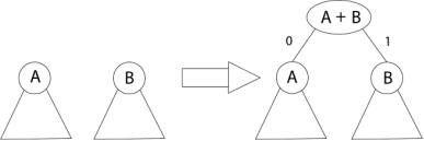
Fig – Greedy Algorithm for constructing a Huffman Code
The algorithm builds the tree T analogous to the optimal code in a bottom-up manner. It starts with a set of |C| leaves (C is the number of characters) and performs |C| - 1 'merging' operations to create the final tree. In the Huffman algorithm 'n' denotes the quantity of a set of characters, z indicates the parent node, and x & y are the left & right child of z respectively.
Huffman (C)
1. n=|C|
2. Q ← C
3. for i=1 to n-1
4. do
5. z= allocate-Node ()
6. x= left[z]=Extract-Min(Q)
7. y= right[z] =Extract-Min(Q)
8. f [z]=f[x]+f[y]
9. Insert (Q, z)
10. return Extract-Min (Q)
Example: Find an optimal Huffman Code for the following set of frequencies:
Solution:
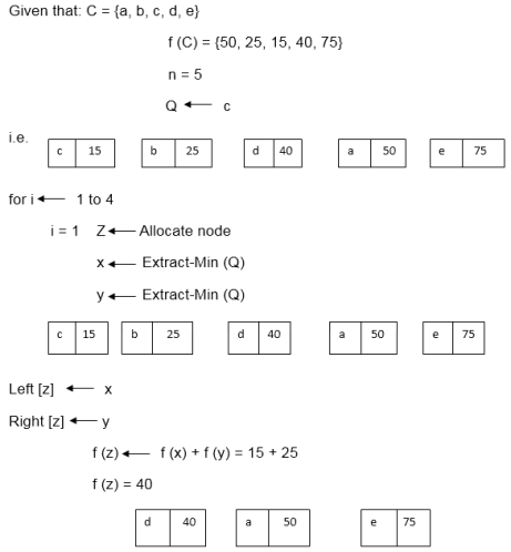
i.e.
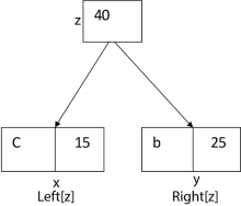
Again, for i=2
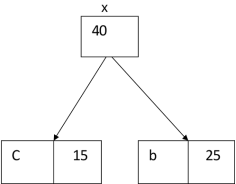
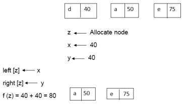
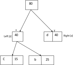
Similarly, we apply the same process we get
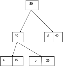
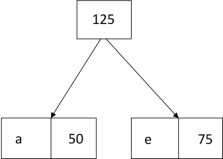
Thus, the final output is:
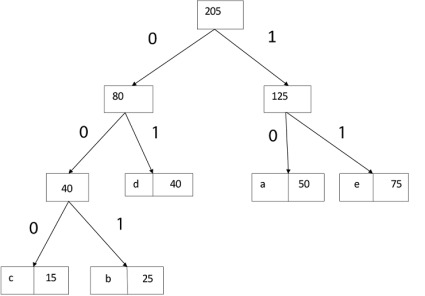
Key takeaways:
(i) Data can be encoded efficiently using Huffman Codes.
(ii) It is a widely used and beneficial technique for compressing data.
(iii) Huffman's greedy algorithm uses a table of the frequencies of occurrences of each character to build up an optimal way of representing each character as a binary string.
Fractional knapsack problem can be solved by Greedy Strategy whereas 0 /1 problem is not.
It cannot be solved by Dynamic Programming Approach.
In this item cannot be broken which means thief should take the item as a whole or should leave it. That's why it is called 0/1 knapsack Problem.
Example of 0/1 Knapsack Problem:
Example: The maximum weight the knapsack can hold is W is 11. There are five items to choose from. Their weights and values are presented in the following table:

The [i, j] entry here will be V [i, j], the best value obtainable using the first "i" rows of items if the maximum capacity were j. We begin by initialization and first row.

V [i, j] = max {V [i - 1, j], vi + V [i - 1, j -wi]


The value of V [3, 7] was computed as follows:
V [3, 7] = max {V [3 - 1, 7], v3 + V [3 - 1, 7 - w3]
= max {V [2, 7], 18 + V [2, 7 - 5]}
= max {7, 18 + 6}
= 24

Finally, the output is:

The maximum value of items in the knapsack is 40, the bottom-right entry). The dynamic programming approach can now be coded as the following algorithm:
KNAPSACK (n, W)
1. for w = 0, W
2. do V [0, w] ← 0
3. for i=0, n
4. do V [i, 0] ← 0
5. for w = 0, W
6. do if (wi≤ w & vi + V [i-1, w - wi]> V [i -1, W])
7. then V [i, W] ← vi + V [i - 1, w - wi]
8. else V [i, W] ← V [i - 1, w]
Key takeaways:
Knapsack is basically means bag. A bag of given capacity.
We want to pack n items in your luggage.
Input:
Output: To maximize profit and minimize weight in capacity.
The activity selection problem is a mathematical optimization problem. Our first illustration is the problem of scheduling a resource among several challenge activities. We find a greedy algorithm provides a well-designed and simple method for selecting a maximum- size set of manually compatible activities.
Suppose S = {1, 2....n} is the set of n proposed activities. The activities share resources which can be used by only one activity at a time, e.g., Tennis Court, Lecture Hall, etc. Each Activity "i" has start time si and a finish time fi, where si ≤fi. If selected activity "i" take place meanwhile the half-open time interval [si, fi). Activities i and j are compatible if the intervals (si, fi) and [si, fi) do not overlap (i.e., i and j are compatible if si ≥fi or si ≥fi). The activity-selection problem chosen the maximum- size set of mutually consistent activities.
Algorithm Of Greedy- Activity Selector:
GREEDY- ACTIVITY SELECTOR (s, f)
1. n ← length [s]
2. A ← {1}
3. j ← 1.
4. for i ← 2 to n
5. do if si ≥ fi
6. then A ← A ∪ {i}
7. j ← i
8. return A
Example: Given 10 activities along with their start and end time as
S = (A1 A2 A3 A4 A5 A6 A7 A8 A9 A10)
Si = (1,2,3,4,7,8,9,9,11,12)
fi = (3,5,4,7,10,9,11,13,12,14)
Compute a schedule where the greatest number of activities takes place.
Solution: The solution to the above Activity scheduling problem using a greedy strategy is illustrated below:
Arranging the activities in increasing order of end time

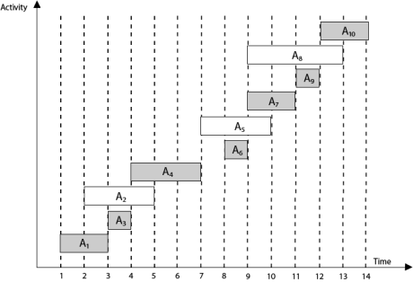
Now, schedule A1
Next schedule A3 as A1 and A3 are non-interfering.
Next skip A2 as it is interfering.
Next, schedule A4 as A1 A3 and A4 are non-interfering, then next, schedule A6 as A1 A3 A4 and A6 are non-interfering.
Skip A5 as it is interfering.
Next, schedule A7 as A1 A3 A4 A6 and A7 are non-interfering.
Next, schedule A9 as A1 A3 A4 A6 A7 and A9 are non-interfering.
Skip A8 as it is interfering.
Next, schedule A10 as A1 A3 A4 A6 A7 A9 and A10 are non-interfering.
Thus, the final Activity schedule is:

Key takeaways:
"Greedy Method finds out of many options, but you have to choose the best option."
In this method, we have to find out the best method/option out of many present ways.
In this approach/method we focus on the first stage and decide the output, don't think about the future.
This method may or may not give the best output.
Dynamic programming approach is similar to divide and conquer in breaking down the problem into smaller and yet smaller possible sub-problems. But unlike, divide and conquer, these sub-problems are not solved independently. Rather, results of these smaller sub-problems are remembered and used for similar or overlapping sub-problems.
Dynamic programming is used where we have problems, which can be divided into similar sub-problems, so that their results can be re-used. Mostly, these algorithms are used for optimization. Before solving the in-hand sub-problem, dynamic algorithm will try to examine the results of the previously solved sub-problems. The solutions of sub-problems are combined in order to achieve the best solution.
So, we can say that −
In contrast to greedy algorithms, where local optimization is addressed, dynamic algorithms are motivated for an overall optimization of the problem.
In contrast to divide and conquer algorithms, where solutions are combined to achieve an overall solution, dynamic algorithms use the output of a smaller sub-problem and then try to optimize a bigger sub-problem. Dynamic algorithms use Memorization to remember the output of already solved sub-problems.
The following computer problems can be solved using dynamic programming approach −
Dynamic programming can be used in both top-down and bottom-up manner. And of course, most of the times, referring to the previous solution output is cheaper than recomputing in terms of CPU cycles.
Key takeaway
Dynamic programming approach is similar to divide and conquer in breaking down the problem into smaller and yet smaller possible sub-problems. But unlike, divide and conquer, these sub-problems are not solved independently. Rather, results of these smaller sub-problems are remembered and used for similar or overlapping sub-problems.
Dynamic programming is used where we have problems, which can be divided into similar sub-problems, so that their results can be re-used. Mostly, these algorithms are used for optimization. Before solving the in-hand sub-problem, dynamic algorithm will try to examine the results of the previously solved sub-problems. The solutions of sub-problems are combined in order to achieve the best solution.
Example: We are given the sequence {4, 10, 3, 12, 20, and 7}. The matrices have size 4 x 10, 10 x 3, 3 x 12, 12 x 20, 20 x 7. We need to compute M [i, j], 0 ≤ i, j≤ 5. We know M [i, i] = 0 for all i.
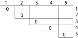
Let us proceed with working away from the diagonal. We compute the optimal solution for the product of 2 matrices.

Here P0 to P5 are Position and M1 to M5 are matrix of size (pi to pi-1)
On the basis of sequence, we make a formula

In Dynamic Programming, initialization of every method done by '0’. So, we initialize it by '0’. It will sort out diagonally.
We have to sort out all the combination but the minimum output combination is taken into consideration.
Calculation of Product of 2 matrices:
1. m (1,2) = m1 x m2
= 4 x 10 x 10 x 3
= 4 x 10 x 3 = 120
2. m (2, 3) = m2 x m3
= 10 x 3 x 3 x 12
= 10 x 3 x 12 = 360
3. m (3, 4) = m3 x m4
= 3 x 12 x 12 x 20
= 3 x 12 x 20 = 720
4. m (4,5) = m4 x m5
= 12 x 20 x 20 x 7
= 12 x 20 x 7 = 1680
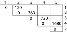
Now the third diagonal will be solved out in the same way.
Now product of 3 matrices:
M [1, 3] = M1 M2 M3

M [1, 3] =264
As Comparing both output 264 is minimum in both cases so we insert 264 in table and (M1 x M2) + M3 this combination is chosen for the output making.
M [2, 4] = M2 M3 M4

M [2, 4] = 1320
As Comparing both output 1320 is minimum in both cases so we insert 1320 in table and M2+(M3 x M4) this combination is chosen for the output making.
M [3, 5] = M3 M4 M5

M [3, 5] = 1140
As Comparing both output 1140 is minimum in both cases so we insert 1140 in table and (M3 x M4) + M5this combination is chosen for the output making.

Now product of 4 matrices:
M [1, 4] = M1 M2 M3 M4
There are three cases by which we can solve this multiplication:
After solving these cases we choose the case in which minimum output is there

M [1, 4] =1080
As comparing the output of different cases then '1080' is minimum output, so we insert 1080 in the table and (M1 xM2) x (M3 x M4) combination is taken out in output making,
M [2, 5] = M2 M3 M4 M5
There are three cases by which we can solve this multiplication:
After solving these cases we choose the case in which minimum output is there

M [2, 5] = 1350
As comparing the output of different cases then '1350' is minimum output, so we insert 1350 in the table and M2 x (M3 x M4 xM5) combination is taken out in output making.

Now product of 5 matrices:
M [1, 5] = M1 M2 M3 M4 M5
There are five cases by which we can solve this multiplication:
After solving these cases we choose the case in which minimum output is there

M [1, 5] = 1344
As comparing the output of different cases then '1344' is minimum output, so we insert 1344 in the table and M1 x M2 x (M3 x M4 x M5) combination is taken out in output making.
Final Output is:

Step 3: Computing Optimal Costs: let us assume that matrix Ai has dimension pi-1x pi for i=1, 2, 3.... n. The input is a sequence (p0, p1, ......pn) where length [p] = n+1. The procedure uses an auxiliary table m [1....n, 1......n] for storing m [i, j] costs an auxiliary table s [1....n, 1......n] that record which index of k achieved the optimal costs in computing m [i, j].
The algorithm first computes m [i, j] ← 0 for i=1, 2, 3......n, the minimum costs for the chain of length 1.
Algorithm of Matrix Chain Multiplication
MATRIX-CHAIN-ORDER (p)
1. n length[p]-1
2. for i ← 1 to n
3. do m [i, i] ← 0
4. for l ← 2 to n // l is the chain length
5. do for i ← 1 to n-l + 1
6. do j ← i+ l -1
7. m [i, j] ← ∞
8. for k ← i to j-1
9. do q ← m [i, k] + m [k + 1, j] + pi-1 pk pj
10. If q < m [i, j]
11. then m [i, j] ← q
12. s [i, j] ← k
13. return m and s.
We will use table s to construct an optimal solution.
Step 1: Constructing an Optimal Solution:
PRINT-OPTIMAL-PARENS (s, i, j)
1. if i=j
2. then print "A"
3. else print "("
4. PRINT-OPTIMAL-PARENS (s, i, s [i, j])
5. PRINT-OPTIMAL-PARENS (s, s [i, j] + 1, j)
6. print ")"
Analysis: There are three nested loops. Each loop executes a maximum n time.
Body of loop constant complexity
Total Complexity is: O (n3)
Algorithm with Explained Example
Question: P [7, 1, 5, 4, 2}
Solution: Here, P is the array of a dimension of matrices.
So here we will have 4 matrices:
A17x1 A21x5 A35x4 A44x2
i.e.
First Matrix A1 have dimension 7 x 1
Second Matrix A2 have dimension 1 x 5
Third Matrix A3 have dimension 5 x 4
Fourth Matrix A4 have dimension 4 x 2
Let say,
From P = {7, 1, 5, 4, 2} - (Given)
And P is the Position
p0 = 7, p1 =1, p2 = 5, p3 = 4, p4=2.
Length of array P = number of elements in P
∴length (p)= 5
From step 3
Follow the steps in Algorithm in Sequence
According to Step 1 of Algorithm Matrix-Chain-Order
Step 1:
n ← length [p]-1
Where n is the total number of elements
And length [p] = 5
∴ n = 5 - 1 = 4
n = 4
Now we construct two tables m and s.
Table m has dimension [1......n, 1.......n]
Table s has dimension [1......n-1, 2.......n]
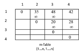
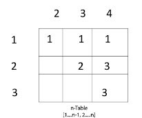
Now, according to step 2 of Algorithm
Case 1:
1. When l - 2
for (i ← 1 to n - l + 1)
i ← 1 to 4 - 2 + 1
i ← 1 to 3
When i = 1
do j ← i + l - 1
j ← 1 + 2 - 1
j ← 2
i.e., j = 2
Now, m [i, j] ← ∞
i.e., m [1,2] ← ∞
Put ∞ in m [1, 2] table
for k ← i to j-1
k ← 1 to 2 - 1
k ← 1 to 1
k = 1
Now q ← m [i, k] + m [k + 1, j] + pi-1 pk pj
for l = 2
i = 1
j =2
k = 1
q ← m [1,1] + m [2,2] + p0x p1x p2
and m [1,1] = 0
for i ← 1 to 4
∴ q ← 0 + 0 + 7 x 1 x 5
q ← 35
We have m [i, j] = m [1, 2] = ∞
Comparing q with m [1, 2]
q < m [i, j]
i.e., 35 < m [1, 2]
35 < ∞
True
then, m [1, 2] ← 35 (∴ m [i, j] ← q)
s [1, 2] ← k
and the value of k = 1
s [1,2] ← 1
Insert "1" at dimension s [1, 2] in table s. And 35 at m [1, 2]
2. l remains 2
L = 2
i ← 1 to n - l + 1
i ← 1 to 4 - 2 + 1
i ← 1 to 3
for i = 1 done before
Now value of i becomes 2
i = 2
j ← i + l - 1
j ← 2 + 2 - 1
j ← 3
j = 3
m [i, j] ← ∞
i.e., m [2,3] ← ∞
Initially insert ∞ at m [2, 3]
Now, for k ← i to j - 1
k ← 2 to 3 - 1
k ← 2 to 2
i.e., k =2
Now, q ← m [i, k] + m [k + 1, j] + pi-1 pk pj
For l =2
i = 2
j = 3
k = 2
q ← m [2, 2] + m [3, 3] + p1x p2 x p3
q ← 0 + 0 + 1 x 5 x 4
q ← 20
Compare q with m [i, j]
If q < m [i, j]
i.e., 20 < m [2, 3]
20 < ∞
True
Then m [i, j] ← q
m [2, 3] ← 20
and s [2, 3] ← k
and k = 2
s [2,3] ← 2
3. Now i become 3
i = 3
l = 2
j ← i + l - 1
j ← 3 + 2 - 1
j ← 4
j = 4
Now, m [i, j] ← ∞
m [3,4] ← ∞
Insert ∞ at m [3, 4]
for k ← i to j - 1
k ← 3 to 4 - 1
k ← 3 to 3
i.e., k = 3
Now, q ← m [i, k] + m [k + 1, j] + pi-1 pk pj
i = 3
l = 2
j = 4
k = 3
q ← m [3, 3] + m [4,4] + p2 x p3 x p4
q ← 0 + 0 + 5 x 2 x 4
q 40
Compare q with m [i, j]
If q < m [i, j]
40 < m [3, 4]
40 < ∞
True
Then, m [i, j] ← q
m [3,4] ← 40
and s [3,4] ← k
s [3,4] ← 3
Case 2: l becomes 3
L = 3
for i = 1 to n - l + 1
i = 1 to 4 - 3 + 1
i = 1 to 2
When i = 1
j ← i + l - 1
j ← 1 + 3 - 1
j ← 3
j = 3
Now, m [i, j] ← ∞
m [1, 3] ← ∞
for k ← i to j - 1
k ← 1 to 3 - 1
k ← 1 to 2
Now we compare the value for both k=1 and k = 2. The minimum of two will be placed in m [i, j] or s [i, j] respectively.
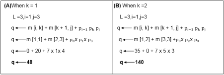
Now from above
Value of q become minimum for k=1
∴ m [i, j] ← q
m [1,3] ← 48
Also, m [i, j] > q
i.e., 48 < ∞
∴ m [i, j] ← q
m [i, j] ← 48
and s [i, j] ← k
i.e., m [1,3] ← 48
s [1, 3] ← 1
Now i become 2
i = 2
l = 3
then j ← i + l -1
j ← 2 + 3 - 1
j ← 4
j = 4
so, m [i, j] ← ∞
m [2,4] ← ∞
Insert initially ∞ at m [2, 4]
for k ← i to j-1
k ← 2 to 4 - 1
k ← 2 to 3
Here, also find the minimum value of m [i, j] for two values of k = 2 and k =3
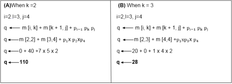
Case 3: l becomes 4
L = 4
For i ← 1 to n-l + 1
i ← 1 to 4 - 4 + 1
i ← 1
i = 1
do j ← i + l - 1
j ← 1 + 4 - 1
j ← 4
j = 4
Now m [i, j] ← ∞
m [1,4] ← ∞
for k ← i to j -1
k ← 1 to 4 - 1
k ← 1 to 3
When k = 1
q ← m [i, k] + m [k + 1, j] + pi-1 pk pj
q ← m [1,1] + m [2,4] + p0xp4x p1
q ← 0 + 28 + 7 x 2 x 1
q ← 42
Compare q and m [i, j]
m [i, j] was ∞
i.e., m [1,4]
if q < m [1,4]
42< ∞
True
Then m [i, j] ← q
m [1,4] ← 42
and s [1,4] 1 ? k =1
When k = 2
L = 4, i=1, j = 4
q ← m [i, k] + m [k + 1, j] + pi-1 pk pj
q ← m [1, 2] + m [3,4] + p0 xp2 xp4
q ← 35 + 40 + 7 x 5 x 2
q ← 145
Compare q and m [i, j]
Now m [i, j]
i.e., m [1,4] contains 42.
So, if q < m [1, 4]
But 145 less than or not equal to m [1, 4]
So, 145 less than or not equal to 42.
So, no change occurs.
When k = 3
l = 4
i = 1
j = 4
q ← m [i, k] + m [k + 1, j] + pi-1 pk pj
q ← m [1, 3] + m [4,4] + p0 xp3 x p4
q ← 48 + 0 + 7 x 4 x 2
q ← 114
Again, q less than or not equal to m [i, j]
i.e., 114 less than or not equal to m [1, 4]
114 less than or not equal to 42
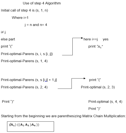
So, no change occurs. So, the value of m [1, 4] remains 42. And value of s [1, 4] = 1
Now we will make use of only s table to get an optimal solution.
A subsequence of a given sequence is just the given sequence with some elements left out.
Given two sequences X and Y, we say that the sequence Z is a common sequence of X and Y if Z is a subsequence of both X and Y.
In the longest common subsequence problem, we are given two sequences X = (x1 x2....xm) and Y = (y1 y2 yn) and wish to find a maximum length common subsequence of X and Y. LCS Problem can be solved using dynamic programming.
Characteristics of Longest Common Sequence
A brute-force approach we find all the sub sequences of X and check each subsequence to see if it is also a subsequence of Y, this approach requires exponential time making it impractical for the long sequence.
Given a sequence X = (x1 x2......xm) we define the ith prefix of X for i=0, 1, and 2...m as Xi= (x1 x2....xi). For example: if X = (A, B, C, B, C, A, B, C) then X4= (A, B, C, B)
Optimal Substructure of an LCS: Let X = (x1 x2....xm) and Y = (y1 y2......) yn) be the sequences and let Z = (z1 z2......zk) be any LCS of X and Y.
Step 2: Recursive Solution: LCS has overlapping subproblems property because to find LCS of X and Y, we may need to find the LCS of Xm-1 and Yn-1. If xm ≠ yn, then we must solve two subproblems finding an LCS of X and Yn-1. Whenever of these LCS's longer is an LCS of x and y. But each of these subproblems has the subproblems of finding the LCS of Xm-1 and Yn-1.
Let c [i, j] be the length of LCS of the sequence Xi and Yj. If either i=0 and j =0, one of the sequences has length 0, so the LCS has length 0. The optimal substructure of the LCS problem given the recurrence formula

Step3: Computing the length of an LCS: let two sequences X = (x1 x2......xm) and Y = (y1 y2...... yn) as inputs. It stores the c [i, j] values in the table c [0......m, 0..........n]. Table b [1..........m, 1..........n] is maintained which help us to construct an optimal solution. c [m, n] contains the length of an LCS of X, Y.
Algorithm of Longest Common Sequence
LCS-LENGTH (X, Y)
1. m ← length
[X]
2. n ← length [Y]
3. for i ← 1 to m
4. do c [i,0] ← 0
5. for j ← 0 to m
6. do c [0, j] ← 0
7. for i ← 1 to m
8. do for j ← 1 to n
9. do if xi= yj
10. then c [i, j] ← c [i-1, j-1] + 1
11. b [i, j] ← "↖"
12. else if c [i-1, j] ≥ c [i, j-1]
13. then c [i, j] ← c [i-1, j]
14. b [i, j] ← "↑"
15. else c [i, j] ← c [i, j-1]
16. b [i, j] ← "← "
17. return c and b.
Example of Longest Common Sequence
Example: Given two sequences X [1...m] and Y [1......n]. Find the longest common sub sequences to both.

here X = (A, B, C, B, D, A, B) and Y = (B, D, C, A, B, A)
m = length [X] and n = length [Y]
m = 7 and n = 6
Here x1= x [1] = A y1= y [1] = B
x2= B y2= D
x3= C y3= C
x4= B y4= A
x5= D y5= B
x6= A y6= A
x7= B
Now fill the values of c [i, j] in m x n table
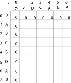
Initially, for i=1 to 7 c [i, 0] = 0
For j = 0 to 6 c [0, j] = 0
That is:
Now for i=1 and j = 1
x1 and y1 we get x1 ≠ y1 i.e. A ≠ B
And c [i-1, j] = c [0, 1] = 0
c [i, j-1] = c [1,0] = 0
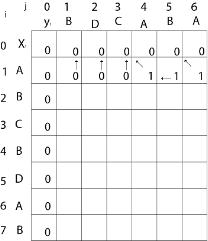
That is, c [i-1, j] = c [i, j-1] so c [1, 1] = 0 and b [1, 1] = ' ↑ ‘
Now for i=1 and j = 2
x1 and y2 we get x1 ≠ y2 i.e. A ≠ D
c [i-1, j] = c [0, 2] = 0
c [i, j-1] = c [1,1] = 0
That is, c [i-1, j] = c [i, j-1] and c [1, 2] = 0 b [1, 2] = ‘↑ ‘
Now for i=1 and j = 3
x1 and y3 we get x1 ≠ y3 i.e. A ≠ C
c [i-1, j] = c [0, 3] = 0
c [i, j-1] = c [1,2] = 0
so, c [1,3] = 0 b [1,3] = ' ↑ '
Now for i=1 and j = 4
x1 and y4 we get. x1=y4 i.e. A = A
c [1,4] = c [1-1,4-1] + 1
= c [0, 3] + 1
= 0 + 1 = 1
c [1,4] = 1
b [1,4] = ‘↖ ‘
Now for i=1 and j = 5
x1 and y5 we get x1 ≠ y5
c [i-1, j] = c [0, 5] = 0
c [i, j-1] = c [1,4] = 1
Thus c [i, j-1] > c [i-1, j] i.e., c [1, 5] = c [i, j-1] = 1. So, b [1, 5] = '←'
Now for i=1 and j = 6
x1 and y6 we get x1=y6
c [1, 6] = c [1-1,6-1] + 1
= c [0, 5] + 1 = 0 + 1 = 1
c [1,6] = 1
b [1,6] = ‘↖ ‘
Now for i=2 and j = 1
We get x2 and y1 B = B i.e. x2= y1
c [2,1] = c [2-1,1-1] + 1
= c [1, 0] + 1
= 0 + 1 = 1
c [2, 1] = 1 and b [2, 1] = ' ↖ '
Similarly, we fill the all values of c [i, j] and we get
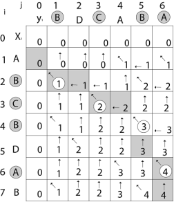
Step 4: Constructing an LCS: The initial call is PRINT-LCS (b, X, X. length, Y. length)
PRINT-LCS (b, x, i, j)
1. if i=0 or j=0
2. then return
3. if b [i, j] = ' ↖ '
4. then PRINT-LCS (b, x, i-1, j-1)
5. print x_i
6. else if b [i, j] = ‘↑ ‘
7. then PRINT-LCS (b, X, i-1, j)
8. else PRINT-LCS (b, X, i, j-1)
Example: Determine the LCS of (1,0,0,1,0,1,0,1) and (0,1,0,1,1,0,1,1,0).
Solution: let X = (1,0,0,1,0,1,0,1) and Y = (0,1,0,1,1,0,1,1,0).

We are looking for c [8, 9]. The following table is built.
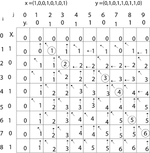
From the table we can deduct that LCS = 6. There are several such sequences, for instance (1,0,0,1,1,0) (0,1,0,1,0,1) and (0,0,1,1,0,1)
In the traveling salesman Problem, a salesman must visit n cities. We can say that salesman wishes to make a tour or Hamiltonian cycle, visiting each city exactly once and finishing at the city he starts from. There is a non-negative cost c (i, j) to travel from the city i to city j. The goal is to find a tour of minimum cost. We assume that every two cities are connected. Such problems are called Traveling-salesman problem (TSP).
We can model the cities as a complete graph of n vertices, where each vertex represents a city.
It can be shown that TSP is NPC.
If we assume the cost function c satisfies the triangle inequality, then we can use the following approximate algorithm.
Let u, v, w be any three vertices, we have

One important observation to develop an approximate solution is if we remove an edge from H*, the tour becomes a spanning tree.
Traveling-salesman Problem
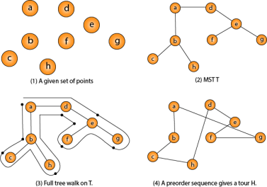
Fig - Traveling-salesman Problem
Intuitively, Approx-TSP first makes a full walk of MST T, which visits each edge exactly two times. To create a Hamiltonian cycle from the full walk, it bypasses some vertices (which corresponds to making a shortcut)
Branch and bound is an algorithm design paradigm which is generally used for solving combinatorial optimization problems. These problems are typically exponential in terms of time complexity and may require exploring all possible permutations in worst case. The Branch and Bound Algorithm technique solves these problems relatively quickly.
Let us consider the 0/1 Knapsack problem to understand Branch and Bound.
There are many algorithms by which the knapsack problem can be solved:
Greedy Algorithm for Fractional Knapsack
DP solution for 0/1 Knapsack
Backtracking Solution for 0/1 Knapsack.
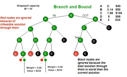
Let’s see the Branch and Bound Approach to solve the 0/1 Knapsack problem: The Backtracking Solution can be optimized if we know a bound on best possible solution subtree rooted with every node. If the best in subtree is worse than current best, we can simply ignore this node and its subtrees. So, we compute bound (best solution) for every node and compare the bound with current best solution before exploring the node.
Example bounds used in below diagram are, A down can give $315, B down can $275, C down can $225, D down can $125 and E down can $30.
Key takeaways:
Specific challenges can be difficult to solve, but they don't have to be excruciating. What you need is the right mindset and a method for solving the dilemma at hand.
Finally, put the solution into use. Is it effective in resolving the issue? Is there anything that you can try?
In case of given m elements of different weights and bins each of capacity C, assign each element to a bin so that number of total implemented bins is minimized. Assumption should be that all elements have weights less than bin capacity.
Input: weight [] = {4, 1, 8, 1, 4, 2}
Bin Capacity c = 10
Output: 2
We require at least 2 bins to accommodate all elements
First bin consists {4, 4, 2} and second bin {8, 2}
We can always calculate a lower bound on minimum number of bins required using ceil () function. The lower bound can be given below −
These algorithms are implemented for Bin Packing problems where elements arrive one at a time (in unknown order), each must be put in a bin, before considering the next element.
Next Fit −
When processing next element, verify if it fits in the same bin as the last element. Implement a new bin only if it does not.
Following is C++ application for this algorithm.
// C++ program to calculate number of bins required implementing next fit algorithm.
#include <bits/stdc++.h>
using namespace std;
// We have to return number of bins needed implementing next fit online algorithm
int nextFit(int weight1[], int m, int C){
// Result (Count of bins) and remaining capacity in current bin are initialized.
int res = 0, bin_rem = C;
// We have to place elements one by one
for (int i = 0; i < m; i++) {
// If this element can't fit in current bin
if (weight1[i] > bin_rem) {
res++; // Use a new bin
bin_rem = C - weight1[i];
}
else
bin_rem -= weight1[i];
}
return res;
}
// Driver program
int main(){
int weight1[] = { 3, 6, 5, 8, 2, 4, 9 };
int C = 10;
int m = sizeof(weight1) / sizeof(weight1[0]);
cout<< "Number of bins required in Next Fit : "
<<nextFit(weight1, m, C);
return 0;
}
Number of bins required in Next Fit : 4
Next Fit is treated as a simple algorithm. It needs only O(m) time and O(1) extra space to process m elements.
First Fit−
When processing the next element, examine or scan the previous bins in order and place the element in the first bin that fits.If element does not fit in any of the existing bins at that time we start a new bin only.
// C++ program to find number of bins needed implementing First Fit algorithm.
#include <bits/stdc++.h>
using namespace std;
// We have to return number of bins needed implementing first fit online algorithm
int firstFit(int weight1[], int m, int C){
// We have to initialize result (Count of bins)
int res = 0;
// We have to create an array to store remaining space in bins there can be maximum n bins
int bin_rem[m];
// We have to place elements one by one
for (int i = 0; i < m; i++) {
// We have to find the first bin that can accommodate weight1[i]
int j;
for (j = 0; j < res; j++) {
if (bin_rem[j] >= weight1[i]) {
bin_rem[j] = bin_rem[j] - weight1[i];
break;
}
}
// If no bin could accommodate weight1[i]
if (j == res) {
bin_rem[res] = C - weight1[i];
res++;
}
}
return res;
}
// Driver program
int main(){
int weight1[] = { 2, 5, 4, 7, 1, 3, 8 };
int C = 10;
int m = sizeof(weight1) / sizeof(weight1[0]);
cout<< "Number of bins required in First Fit : "
<<firstFit(weight1, m, C);
return 0;
}
Number of bins required in First Fit: 4
The above implementation of First Fit consumes O(m2) time, but First Fit can be used in O (m log m) time implementing Self-Balancing Binary Search Trees.
Best Fit −
The concept is to places the next item in the tightest position. That means put it in the bin so that at least empty space is left.
// C++ program to calculate number of bins required implementing Best fit algorithm.
#include <bits/stdc++.h>
using namespace std;
// We have to returns number of bins required implementing best fit online algorithm
int bestFit(int weight1[], int m, int C){
// We have to initialize result (Count of bins)
int res = 0;
// We have to create an array to store remaining space in bins there can be maximum n bins
int bin_rem[m];
// Place elements one by one
for (int i = 0; i < m; i++) {
// Find the best bin that can accomodate weight1[i]
int j;
// We have to initialize minimum space left and index of best bin
int min = C + 1, bi = 0;
for (j = 0; j < res; j++){
if (bin_rem[j] >= weight1[i] && bin_rem[j] - weight1[i] < min) {
bi = j;
min = bin_rem[j] - weight1[i];
}
}
// We create a new bin,if no bin could accommodate weight1[i],
if (min == C + 1) {
bin_rem[res] = C - weight1[i];
res++;
}
else // Assign the element to best bin
bin_rem[bi] -= weight1[i];
}
return res;
}
// Driver program
int main(){
int weight1[] = { 2, 5, 4, 7, 1, 3, 8 };
int C = 10;
int m = sizeof(weight1) / sizeof(weight1[0]);
cout<< "Number of bins required in Best Fit: "
<<bestFit(weight1, m, C);
return 0;
}
Number of bins required in Best Fit: 4
Best Fit can also be applied in O (m log m) time implementing Self-Balancing Binary Search Trees.
In case of the offline version, we have all elements upfront. A problem with online algorithms is that packing large elements is difficult, especially if they occur late in the sequence. We can overcome this by sorting the input sequence, and placing the large elements first.
First Fit Decreasing −
// C++ program to locate number of bins needed implementing First Fit Decreasing algorithm.
#include <bits/stdc++.h>
using namespace std;
/* We copy firstFit() from above */
int firstFit(int weight1[], int m, int C){
// We have to initialize result (Count of bins)
int res = 0;
// We have to create an array to store remaining space in bins there can be maximum n bins
int bin_rem[m];
// We have to place elements one by one
for (int i = 0; i < m; i++) {
// We have to find the first bin that can accommodate weight1[i]
int j;
for (j = 0; j < res; j++) {
if (bin_rem[j] >= weight1[i]) {
bin_rem[j] = bin_rem[j] - weight1[i];
break;
}
}
// If no bin could accommodate weight1[i]
if (j == res) {
bin_rem[res] = C - weight1[i];
res++;
}
}
return res;
}
// We have to returns number of bins required implementing first fit decreasing offline algorithm
int firstFitDec(int weight1[], int m, int C){
// At first we sort all weights in decreasing order
sort(weight1, weight1 + m, std::greater<int>());
// Now we call first fit for sorted items
return firstFit(weight1, m, C);
}
// Driver program
int main(){
int weight1[] = { 2, 5, 4, 7, 1, 3, 8 };
int C = 10;
int m = sizeof(weight1) / sizeof(weight1[0]);
cout<< "Number of bins required in First Fit "
<< "Decreasing: " << firstFitDec(weight1, m, C);
return 0;
}
Number of bins required in First Fit Decreasing: 3
First Fit decreasing generates the best result for the sample input as elements are sorted first.
First Fit Decreasing can also be used in O (m log m) time implementing Self-Balancing Binary Search Trees.
C++ Program to Implement the Bin Packing Algorithm
The bin packing problem is a special type of cutting stock problem. In the bin packing problem, objects of different volumes must be packed into a finite number of containers or bins each of volume V in a way that minimizes the number of bins used. In computational complexity theory, it is a combinational NP-hard problem.
When the number of bins is restricted to 1 and each item is characterized by both a volume and a value, the problem of maximizing the value of items that can fit in the bin is known as the knapsack problem.
Begin
Binpacking(pointer, size, no of sets)
Declare bincount, m, i
Initialize bincount = 1, m=size
For i = 0 to number of sets
if (m - *(a + i) > 0) do
m = m - *(a + i)
Continue
Else
Increase bincount
m = size;
Decrement i
Print number of bins required
End
#include<iostream>
using namespace std;
void binPacking(int *a, int size, int n) {
int binCount = 1;
int m = size;
for (int i = 0; i < n; i++) {
if (m - *(a + i) > 0) {
m -= *(a + i);
continue;
} else {
binCount++;
m = size;
i--;
}
}
cout << "Number of bins required: " << binCount;
}
int main(int argc, char **argv) {
cout << "Enter the number of items in Set: ";
int n;
cin >> n;
cout << "Enter " << n << " items:";
int a[n];
for (int i = 0; i < n; i++)
cin >> a[i];
cout << "Enter the bin size: ";
int size;
cin >> size;
binPacking(a, size, n);
}
Enter the number of items in Set: 3
Enter 3 items:4
6
7
Enter the bin size: 26
Number of bins required: 1
The Traveling Salesman Dilemma (TSP) is to find the shortest possible route that visits each city exactly once and returns to the starting point given a range of cities and distance between each pair of cities.
Take note of the distinction between the Hamiltonian Cycle and the TSP. The Hamiltonian cycle dilemma entails determining if a tour exists that tours each city precisely once. The challenge is to find a minimum weight Hamiltonian Cycle. We know that Hamiltonian Tours exist (because the graph is complete), and there are several of them.
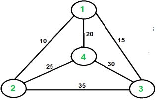
Fig: TSP
Take, for example, the graph in the right-hand figure. In the table, a TSP tour is 1-2-4-3-1. The total expense of the trip is 80 dollars, and is made up of 10 dollars, 25 dollars, 30 dollars, and 15 dollars.
The issue is a well-known NP-hard problem. This problem has no known polynomial time solution.
The following are several solutions to the issue of the travelling salesman.
The informed search algorithm is more useful for large search space. Informed search algorithm uses the idea of heuristic, so it is also called Heuristic search.
Heuristics function: Heuristic is a function which is used in Informed Search, and it finds the most promising path. It takes the current state of the agent as its input and produces the estimation of how close agent is from the goal. The heuristic method, however, might not always give the best solution, but it guaranteed to find a good solution in reasonable time. Heuristic function estimates how close a state is to the goal. It is represented by h(n), and it calculates the cost of an optimal path between the pair of states. The value of the heuristic function is always positive.
Admissibility of the heuristic function is given as:
Here h(n) is heuristic cost, and h*(n) is the estimated cost. Hence heuristic cost should be less than or equal to the estimated cost.
Pure heuristic search is the simplest form of heuristic search algorithms. It expands nodes based on their heuristic value h(n). It maintains two lists, OPEN and CLOSED list. In the CLOSED list, it places those nodes which have already expanded and in the OPEN list, it places nodes which have yet not been expanded.
On each iteration, each node n with the lowest heuristic value is expanded and generates all its successors and n is placed to the closed list. The algorithm continues unit a goal state is found.
In the informed search we will discuss two main algorithms which are given below:
Best First Search Algorithm (Greedy search)
A* Search Algorithm
1.) Best-first Search Algorithm (Greedy Search):
Greedy best-first search algorithm always selects the path which appears best at that moment. It is the combination of depth-first search and breadth-first search algorithms. It uses the heuristic function and search. Best-first search allows us to take the advantages of both algorithms. With the help of best-first search, at each step, we can choose the most promising node. In the best first search algorithm, we expand the node which is closest to the goal node and the closest cost is estimated by heuristic function, i.e.
Were, h(n)= estimated cost from node n to the goal.
The greedy best first algorithm is implemented by the priority queue.
Consider the below search problem, and we will traverse it using greedy best-first search. At each iteration, each node is expanded using evaluation function f(n)=h(n), which is given in the below table.
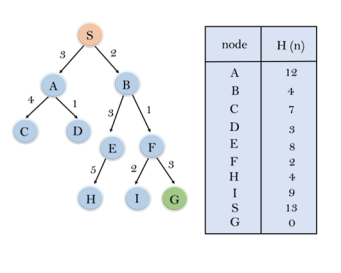
In this search example, we are using two lists which are OPEN and CLOSED Lists. Following is the iteration for traversing the above example.
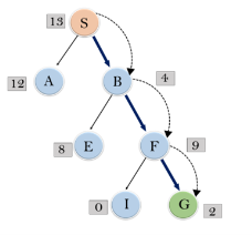
Expand the nodes of S and put in the CLOSED list
Initialization: Open [A, B], Closed [S]
Iteration 1: Open [A], Closed [S, B]
Iteration 2: Open [E, F, A], Closed [S, B]
: Open [E, A], Closed [S, B, F]
Iteration 3: Open [I, G, E, A], Closed [S, B, F]
: Open [I, E, A], Closed [S, B, F, G]
Hence the final solution path will be: S----> B----->F----> G
Time Complexity: The worst-case time complexity of Greedy best first search is O(bm).
Space Complexity: The worst-case space complexity of Greedy best first search is O(bm). Where, m is the maximum depth of the search space.
Complete: Greedy best-first search is also incomplete, even if the given state space is finite.
Optimal: Greedy best first search algorithm is not optimal.
A* search is the most commonly known form of best-first search. It uses heuristic function h(n), and cost to reach the node n from the start state g(n). It has combined features of UCS and greedy best-first search, by which it solves the problem efficiently. A* search algorithm finds the shortest path through the search space using the heuristic function. This search algorithm expands less search tree and provides optimal result faster. A* algorithm is similar to UCS except that it uses g(n)+h(n) instead of g(n).
In A* search algorithm, we use search heuristic as well as the cost to reach the node. Hence, we can combine both costs as following, and this sum is called as a fitness number.

At each point in the search space, only that node is expanded which have the lowest value of f(n), and the algorithm terminates when the goal node is found.
Step1: Place the starting node in the OPEN list.
Step 2: Check if the OPEN list is empty or not, if the list is empty then return failure and stops.
Step 3: Select the node from the OPEN list which has the smallest value of evaluation function (g+h), if node n is goal node, then return success and stop, otherwise
Step 4: Expand node n and generate all of its successors, and put n into the closed list. For each successor n', check whether n' is already in the OPEN or CLOSED list, if not then compute evaluation function for n' and place into Open list.
Step 5: Else if node n' is already in OPEN and CLOSED, then it should be attached to the back pointer which reflects the lowest g(n') value.
Step 6: Return to Step 2.
In this example, we will traverse the given graph using the A* algorithm. The heuristic value of all states is given in the below table so we will calculate the f(n) of each state using the formula f(n)= g(n) + h(n), where g(n) is the cost to reach any node from start state.
Here we will use OPEN and CLOSED list.
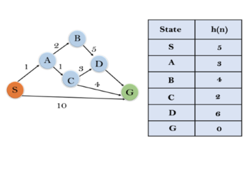
Solution:
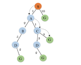
Initialization: {(S, 5)}
Iteration1: {(S--> A, 4), (S-->G, 10)}
Iteration2: {(S--> A-->C, 4), (S--> A-->B, 7), (S-->G, 10)}
Iteration3: {(S--> A-->C--->G, 6), (S--> A-->C--->D, 11), (S--> A-->B, 7), (S-->G, 10)}
Iteration 4 will give the final result, as S--->A--->C--->G it provides the optimal path with cost 6.
Points to remember:
Complete: A* algorithm is complete as long as:
Optimal: A* search algorithm is optimal if it follows below two conditions:
If the heuristic function is admissible, then A* tree search will always find the least cost path.
Time Complexity: The time complexity of A* search algorithm depends on heuristic function, and the number of nodes expanded is exponential to the depth of solution d. So, the time complexity is O(b^d), where b is the branching factor.
Space Complexity: The space complexity of A* search algorithm is O(b^d)
Key takeaways:
Heuristics function: Heuristic is a function which is used in Informed Search, and it finds the most promising path. It takes the current state of the agent as its input and produces the estimation of how close agent is from the goal. The heuristic method, however, might not always give the best solution, but it guaranteed to find a good solution in reasonable time. Heuristic function estimates how close a state is to the goal. It is represented by h(n), and it calculates the cost of an optimal path between the pair of states. The value of the heuristic function is always positive.
1. Introduction to Algorithms, 4TH Edition, Thomas H Cormen, Charles E Lieserson, Ronald L Rivest and Clifford Stein, MIT Press/McGraw-Hill.
2. Fundamentals of Algorithms – E. Horowitz et al.
3. Design and Analysis of Algorithms, M.R.Kabat, PHI Learning
4. Algorithm Design, 1ST Edition, Jon Kleinberg and ÉvaTardos, Pearson.
5. Algorithm Design: Foundations, Analysis, and Internet Examples, Second Edition, Michael T Goodrich and Roberto Tamassia, Wiley.
6. Algorithms—A Creative Approach, 3RD Edition, UdiManber, Addison-Wesley,
Reading, MA.