Unit - 5
Advanced Topics
An Approximate Algorithm is a way of approaching the optimization problem of NP-COMPLETENESS. This approach does not guarantee the right solution. The purpose of an approximation algorithm is to get as close as possible in a reasonable amount of time to the optimum value, which is at the most polynomial moment. These algorithms are called approximation algorithms or heuristic algorithms.
● The optimization issue is to find the shortest cycle for the travelling salesperson problem, and the approximation issue is to find a short cycle.
● The optimization problem for the vertex cover problem is finding the vertex cover with the fewest vertices, and the approximation problem is finding the vertex cover with the fewest vertices.
An algorithm A is said to be an algorithm, given an optimization problem P.
Approximation algorithm for P if it returns an approximation algorithm for any given instance I, approximate solution, that is a feasible solution.
Types of Approximation
P An optimization problem
A An approximation algorithm
I An instance of P
A∗ (I) Optimal value for the instance I
A(I) Value for the instance I generated by A
● A is an absolute approximation algorithm if a constant k exists. Such that I, of P, for every case, |A∗ (I) − A(I)| ≤ k.
● Planar graph colouring, for instance.
2. Relative Approximation
● A is a relative approximation algorithm if there exists a constant k Such that I, of P, for every case, 
● Vertex cover
Example:
1. Vertex Cover
2. Traveling Salesman Problem
3. Bin Packing
Key takeaways:
A vertex cover (or node cover) of a graph is a set of vertices that contains at least one endpoint of each edge of the graph in the mathematical discipline of graph theory. The challenge of finding a minimal vertex cover is a classic computer science optimization problem and a good example of an NP-hard optimization problem with an approximation algorithm. The vertex cover problem, which is a decision variant of the problem, was one of Karp's 21 NP-complete problems and is thus a classic NP-complete problem in computational complexity theory. In addition, the vertex cover problem is a key problem in parameterized complexity theory and is tractable with fixed parameters.
A vertex cover of an undirected graph is a subset of its vertices such that either ‘u' or ‘v' is in the vertex cover for any graph edge (u, v). Despite its name, the Vertex Cover set encompasses all of the graph's edges. The vertex cover problem is to find the smallest vertex cover for an undirected graph.
The explanations below are only a few.

The Vertex Cover Problem is a well-known NP Complete problem, which means that since P = NP, there is no polynomial-time solution. However, there are approximate polynomial-time algorithms that can be used to solve the problem. A basic approximate algorithm adapted from the CLRS book as shown below.
In the traveling salesman Problem, a salesman must visit n cities. We can say that salesman wishes to make a tour or Hamiltonian cycle, visiting each city exactly once and finishing at the city he starts from. There is a non-negative cost c (i, j) to travel from the city i to city j. The goal is to find a tour of minimum cost. We assume that every two cities are connected. Such problems are called Traveling-salesman problem (TSP).
We can model the cities as a complete graph of n vertices, where each vertex represents a city.
It can be shown that TSP is NPC.
If we assume the cost function c satisfies the triangle inequality, then we can use the following approximate algorithm.
Let u, v, w be any three vertices, we have

One important observation to develop an approximate solution is if we remove an edge from H*, the tour becomes a spanning tree.
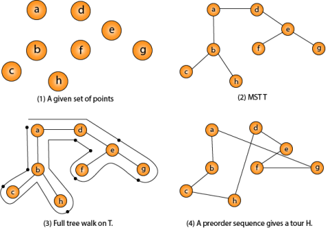
Traveling-salesman Problem

Fig 1 - Traveling-salesman Problem
Intuitively, Approx-TSP first makes a full walk of MST T, which visits each edge exactly two times. To create a Hamiltonian cycle from the full walk, it bypasses some vertices (which corresponds to making a shortcut)
Randomized Algorithms use random numbers in order to decide what should be the next step to be performed. An example of the random algorithm can be like suppose there is a group of students in class and a professor is randomly making a student stand to answer the question.
Randomized algorithms sometimes have deterministic time complexity. Algorithms like Monte Carlo algorithm use a randomized approach and its worst-case complexity can be easily identified, whereas randomized algorithms like Las Vegas are dependent on the value of random variables and hence in these algorithms worst case identification becomes tougher.
In order to compute expected time taken in the worst case a time taken by every possible value needs to be evaluated. Average of all evaluated times is the expected worst case time complexity
Randomized algorithm is mainly used either to reduce the time complexity or the space complexity in the given algorithm
Randomized algorithms are classified into two categories
Example of Las Vegas
Finding Random point in the circle
It is easy and convenient to find a random point in the circle using this approach, here the idea is to first generate a point (x, y) with -1< x <1 and -1<y <1. So, if the random selected point appears in this unit circle, we keep it else we will throw it and repeat until the point in the unit circle is found
Algorithm for finding Random point in the circle
funpoint()(x,y float64)
{
for
{
x=2* rand.Float64()-1
y=2* rand.Float64()-1
if x*x+y*y < 1
{
Return
}
}
}
2. Monte Carlo: - These algorithms produce the correct or optimum result on the basis of probability. Monte Carlo algorithm has deterministic running time and it is generally easier to find out worst case time complexity.
For example, implementation of Karger’s algorithm produces a minimum cut with probability greater than or equal to (1/n2) where n is the number of vertices in Karger’s algorithm and it has the worst-case time complexity as O(E).
Monte Carlo simulations are a broad class of algorithms that use repeated random sampling to obtain numerical results; these are generally used to simulate the behavior of other systems.
If a point (x, y) with -1< x <1 and -1<y <1 is placed randomly then the ratio of points that fall within the unit circle will be close to.
Algorithm to find a random point in the given circle using Monte Carlo approach
const a = 99999
count: = 0
for i: = 0; i <a; i++ {
x: = 2*rand.Float64() - 1
y: = 2*rand.Float64() - 1
if x*x+y*y < 1 {
count++
}
}
Key takeaways:
Quick sort is an extremely efficient sorting technique that divides a large data array into smaller ones. A huge array is divided into two arrays, one of which contains values lower than the provided value, say pivot, on which the partition is based, and the other of which contains values bigger than the pivot value.
Quicksort divides an array into two subarrays and then calls itself recursively twice to sort the two subarrays. Because the average and worst-case complexity of this approach are O(n2), it is very efficient for huge data sets.
Algorithm for Quick Sort Pivot
We'll try to create an algorithm for partitioning in rapid sort based on our knowledge of it, which is as follows.
Step 1: Decide which index value has the highest pivot.
Step 2: Exclude the pivot and use two variables to point left and right of the list.
Step 3 to the left indicates the low index.
Step 4: The right arrow points to the highest place.
Step 5: Move right when the value at the left is smaller than the pivot.
Step 6: Move left when the value at the right is bigger than the pivot.
Step 7: Swap left and right if both steps 5 and 6 don't match.
Step 8: If they meet on the left or right, the place where they met becomes the new pivot.
Algorithm for Quick Sorting
We get smaller potential divisions by iteratively using the pivot approach. After that, each division is processed for speedy sorting. The recursive algorithm for quicksort is defined as follows:
Step 1: Pivot the index value that is farthest to the right.
Step 2: Using the pivot value, split the array.
Step 3: Recursively quicksort the left partition
Step 4: Recursively quicksort the right partition
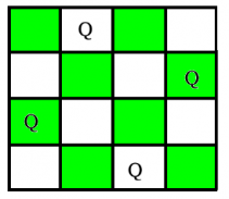
The N Queen problem is the task of arranging N chess queens on a NN chessboard in such a way that no two queens attack one other. For instance, here is a solution to the 4 Queens problem.
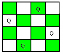
The N Queen problem is the task of arranging N chess queens on a NN chessboard in such a way that no two queens attack one other. The four-queen issue, for example, has two solutions.


After discussing a strategy that publishes only one potential answer in the previous article, the aim in this article is to publish all solutions in the N-Queen Problem.
Each solution is a permutation of [1,2, 3...n] in increasing order, with the number in the ith position indicating that the ith-column queen is put in the row with that number. [[2 4 1 3] [3 1 4 2]] is the solution for the scenario above. The methodology used in this solution is an extension of that method.
The minimal sum of weights of (at least one) edges that, when removed from the graph, separates the graph into two groups is known as the Min-Cut of a weighted graph. In 1995, Mechthild Stoer and Frank Wagner devised a method for determining the smallest cut in undirected weighted graphs.
The technique uses a way of decreasing the network by merging the most strongly linked vertex until only one node remains, and the weight of the merged cut is maintained in a list for each step done. The graph's minimal cut value would equal the list's minimum value.
The category of problems that can be solved using just polynomial space.
Exponential (or super-exponential) time is acceptable.
The main point is this:
• Unlike time, space can be reused.
• As a result, PSPACE has a large number of exponential algorithms.
• Take into account universal formulae.
In polynomial space, we may verify them by rerunning the same calculation (say, check(v)) for each v.
•The check area is reused, but the time for different v's adds up.
Please keep in mind that
• PSPACE is where the SAT is. For variables, try every possible truth assignment.
• As a result, PSPACE contains all NP-complete problems.
References:
1. Introduction to Algorithms, 4TH Edition, Thomas H Cormen, Charles E Lieserson, Ronald L Rivest and Clifford Stein, MIT Press/McGraw-Hill.
2. Fundamentals of Algorithms – E. Horowitz et al.
3. Design and Analysis of Algorithms, M.R.Kabat, PHI Learning
4. Algorithm Design, 1ST Edition, Jon Kleinberg and ÉvaTardos, Pearson.
5. Algorithm Design: Foundations, Analysis, and Internet Examples, Second Edition, Michael T Goodrich and Roberto Tamassia, Wiley.
6. Algorithms—A Creative Approach, 3RD Edition, UdiManber, Addison-Wesley,
Reading, MA.