Unit - 5
Concepts of state variables
The state of a system is a minimal set of variables known as state variables. The knowledge of these variables at any instance of time together with the knowledge of the inputs for the same instance of time, determines the complete behaviour of the system. The fewer drawbacks in the transfer function method for representing any system led to the use of state variables in analysis of system. Few advantages are listed below:
- The state space can be used for linear or nonlinear, time-variant or time-invariant systems.
- It is easier to apply where Laplace transform cannot be applied.
- The nth order differential equation can be expressed as 'n' equation of first order.
- It is a time domain method.
- As this is time domain method, therefore this method is suitable for digital computer computation.
- On the basis of the given performance index, this system can be designed for an optimal condition.
Representation of state space: The system shown below has ‘m’ inputs, ‘p, outputs and ‘n’ number of state variables. The state equation gives us the relation between the state variables and the inputs.

So, the above system shown can be described through equations as
 =f1 (x1, x2,…….xn , u1, u2……… ,um)
 = f2 (x1, x2,…….xn , u1, u2……… ,um)
 =f1 (x1, x2,…….xn , u1, u2……… ,um) (1)
The above set of equations can be represented as
 =f(x(t), u(t)) (2)
As we are concerned for time invariant system, for which the term  in (1) is linear combination of state variables and input. So,
 (t)=2tx1+x2+u1+u2 (3)
 =a11x1(t)+a12x2(t)+…a1nxn(t)+b11u1(t)+b12u2(t)+……. +b1mum(t)
 =a21x1(t)+a22x2(t)+…a2nxn(t)+b21u1(t)+b22u2(t)+……. +b2mum(t)
 =an1x1(t)+an2x2(t)+…annxn(t)+bn1u1(t)+bn2u2(t)+……. +bnmum(t)
The above equation can be represented in matrix form as given below
 (4)
(4)
The above coefficients aij and bji in equation (4) can be written in vector matrix form as
 =Ax(t)+Bu(t) (5)
The output of the system can be represented by linear combination of state variables and inputs.
y1=c11x1(t)+c12x2(t)+……. +c1nxn+d11u1+………. +d1mum
y2=c21x1(t)+c22x2(t)+……. +c2nxn+d21u1+………. +d2mum
yr=cr1x1(t)+cr2x2(t)+……. +crnxn+dr1u1+………. +drmum (6)
The equation (6) can be represented in matrix form as
 (7)
(7)
Where coefficients cij and dji are constants. The output equation is given as
Y=CX+DU (8)
Key takeaway
The output equation is given as
Y=CX+DU
The state variables in matrix form can be represented as
 =Ax(t)+Bu(t)
Examples
Q1) Obtatin the state space representation for the given electrical system
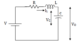
Solution: The state model is given as

The state model shows that there are two energy storing elements L, C. As we already know that Number of state variables is equal to the number of energy storing elements.Hence we have two state variables[x1(t) and x2(t)]. We have one output V0(taken across capacitor) and input u(t).
The output equation is then given as
Y(t)=CX(t)+DU(t)
V0=Vc= x1(t) ….(a)
Hence output equation becomes
V0= x1(t)
y(t)=[1 0] +[0]u(t)
So, C=[1 0] D=[0]
Now writing the state equation
 =Ax(t)+Bu(t)
For that applying KVL in the above circuit
V=ILR+L +Vc
+Vc
State Equation is  =Ax(t)+Bu(t)
 =
=
x1(t)=Vc
 =
=
IL=C
 =
=
 =
= =
=
 =(1/C) x2(t) ……….(b)
 =
= =
=
VL=L
 =
= =VL/L
=VL/L
From KVL
L =VL=V-ILR-VC
 =
= =
=
 =
= …………….(c)
From equation (b) and (c)
 = [0 1/c]
 + [0 0] u(t)
 =[-1/L -R/L]
 + [1/L 0]
Now writing the state equation
 =Ax(t)+Bu(t)
 =
= +
+ 
Hence A= B=
B= 
Q2) Obtatin the state space representation for the given electircal system
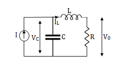
Solution: The state model shows that there are two energy storing elements L, C. As we already know that Number of state variables is equal to the number of energy storing elements.Hence we have two state variables[x1(t) and x2(t)]. We have one output V0(taken across capacitor) and input u(t).
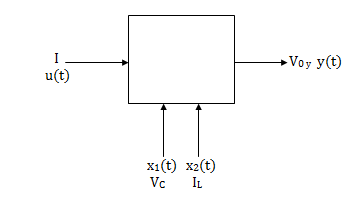
Here output is V0. But from above electrical circuit V0=ILR
V0=x2(t)R
y(t)= V0= [0 R]  + [0] u(t)
The output equation is given as
Y(t)=CX(t)+DU(t)
C=[0 R] D=[0]
Now finding state equation,we apply KCL in the given electrical circuit
I=IC+IL
 =
=
But I-IL=IC
 =
=
 =
=
 =
=
 =
= x2(t)+
 ……..(a)
 =[0 1/C]
 + [1/C 0]
 …….(b)
 =
= =
=
Applying KVL in the given electrical circuit we get
VC=VL+ILR
VC-ILR=VL=L

 =
=
 = [1/L -R/L]
  + [0] u(t) …………. (c)
From equation (b) and (c) we have
Now writing the state equation
 =Ax(t)+Bu(t)
 =
= +
+ 
Hence A= B=
B= 
Note: We should always take voltage across the inductor L, and current through capacitor C.
Q3) Write the state equation for the mechanical system shown below?
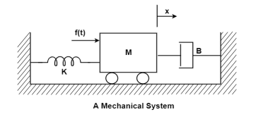
The free body diagram is

The position and velocity are state variables hence,
x1(t)=x(t)
x2(t)= 
 =
= =x2(t)
 =
=
The system equation will be

 =
=
 =
=
 =
=
The state equations are
 = x2(t)
 =
=
 =
= +
+ f(t)
f(t)
Q4) The closed loop transfer function is given as T(s)= . Calculate the state model?
Sol: The transfer function can be simplified using partial fraction method as
 =
=
S+2=As+10A+Bs+5B
Equating coefficients of s from both sides
A+B=1
Equating coefficients of s0 from both sides
10A+5B=2
Solving above equations we get
A=-3/5
B=8/5
The transfer function will be
T(s)=
=- +
+
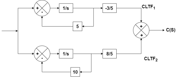
Number of poles= Number of energy storing elements
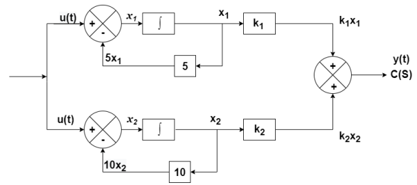
The output equation is given as
y(t)=k1x1(t)+k2x2(t)
y(t)= [k1 k2] + [0] [u(t)]
y(t)= [-3/5 8/5] + [0] [u(t)]
C= [-3/5 8/5]
D=0
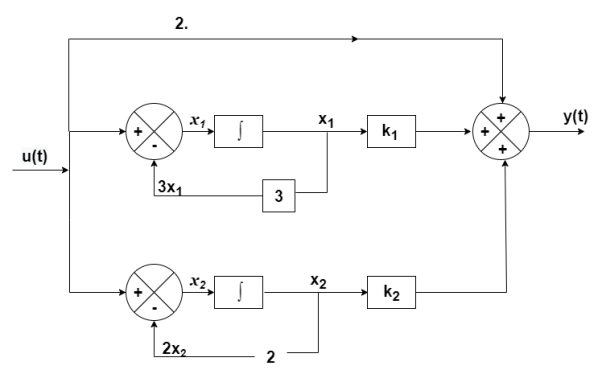
From the above block diagram
 =u(t)-5 x1
 =-5x1+u(t)
 =-10x2+u
Therefore, the state equation is given as
 =
= +
+
A=
B=
Q5) The closed loop transfer function is given as T(s)= . Calculate the state model?
Sol: The transfer function can be simplified using partial fraction method as
 =
= +
+ 
s+7=A[s2+7s+12] +B[s2+6s+8] +C[s2+5s+6]
Equating coefficients of s2 from both sides
A+B+C=0
Equating coefficients of s from both sides
7A+6B+5C=1
Equating coefficients of s0 from both sides
12A+8B+6C=7
Solving above equations and finding values of A, B and C
A=5/2
B=-4
C=3/2
The transfer function will be
T(s)= +
+ 
= +
+ 
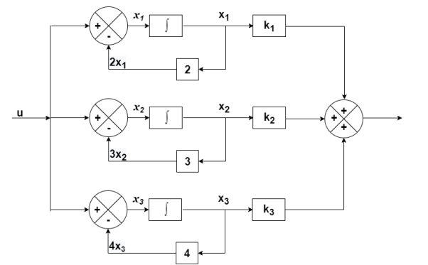
The output equation will be
y=k1x1+k2x2+k3x3
y= [k1 k2 k3] [5/2 -4 3/2]
C= [5/2 -4 3/2]
D= [0]
The state equation is given as
 =u(t)-2x1
 =-2x1+u(t)
 =-3x2+u
 = -4x3+u
Therefore
 =
= +
+ [u]
[u]
A=
B=
Q6) The closed loop transfer function is T(s)= . Find the state equation?
Sol: Here the number of poles = number of zeros
T(s)=
=
=
=2+ 
=2+
Solving above by partial fraction method
88= As+2A+Bs+3B
A=-B
2A+3B=88
A=-88
B=88
The transfer function becomes
T(s)= 2-
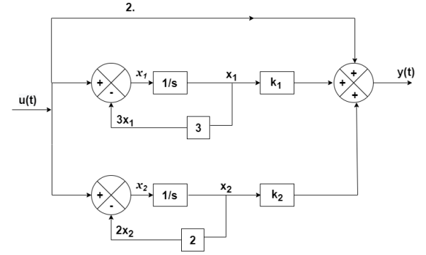
The output equation will be
y(t)=2U+k1x1+k2x2
y= [-88 88] + [2]u
The output equation will be
 =u(t)-3 x1
 =-3x1+u(t)
 =-2x2+u(t)
Therefore, the state equation is given as
 =
= +
+
A=
B=
Q7) The CLTF T(s)= . Find the state equation?
Sol: T(s)=
=
P1=2/s
P2=-8/s2
L1=-10/s
L2=-100/s2
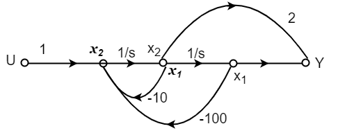
The state equation will be
 =x2
=x2
 =-10x2-100x1+u
 =
= +
+
Q8) Find the state equation from the given differential equation

Sol: Let y=x1
 =
= =x2
=x2
 =
= =x3
=x3
 =
=
The above differential equation than becomes
 +6
+6 +11 x2+6 x1=u
 (t) =u-6
 (t)-11 x2-6 x1
Hence the state equation will be
 =
=  +
+ [u]
[u]
Q9) For the given data below compute the transfer function of the system
A= B=
B= C= [1 0] and D= [0]
Sol: The state equation will be
 =
= +
+
 =x1
=x1
 =-6x1-5x2
Equation (14) in section 4.1
 = C{[SI-A]-1B} + D
=C { -
- }-1B+D
=C B+D
B+D
= [1 0] 
 + 0
+ 0
= +0
+0
 =
=
Q10) Obtain the state space representation of following mechanical system

Sol: The position and velocity state variables will be
x1=y1
x2=
x3=y2
x4=
The difference equation will be
M1 +B1
+B1 +K1y1+B2(
 -
- +K2(y1-y2) =0
M2 + K2(y2-y1) + B2(
 -
- )=u
)=u
Writing above equations in the form of state variables
M2 =u-K2(y2-y1) +-B2(
 -
- )
)
M1 =- B1
=- B1 -K1y1-B2(
 -
- -K2(y1-y2)
 = -(
= -( +
+ )x1- (
 ) x2+(
 )x3+
)x3+ x4
x4
 =
=  x1+
x1+ x2-
x2- x3-
x3- x4+
x4+
Now writing all the state equations
 =x2
=x2
 = -(
= -( +
+ )x1- (
 ) x2+(
 )x3+
)x3+ x4
x4
 = x4
= x4
 =
=  x1+
x1+ x2-
x2- x3-
x3- x4+
x4+
The matrix form for above equations is given below
 =
= 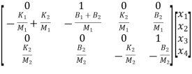 +
+ v(t)
v(t)
Diagonalization
A diagonal system matrix has an advantage that each state equation is the function of only one state variable. Hence, each state equation can be solved simultaneously. The technique of transforming a non-diagonal matrix to diagonal matrix is known as diagonalization.
The state equation is given as

Y(t)=Cx(t)+Du(t)
Let the eigen values of matrix A be  1,
1, 2,
2, 3 …… Then Let us transform X into a new state vector Z
X=PZ
P is n x m non-singular matrix
P =APZ+BU
Y=CPZ+DU
 =
= Z+
Z+ U
U
Y= Z+
Z+ U
U
 =P-1AP
 = P-1B
 =CP
=CP
Diagonalization of system matrices with distinct and repeated eigen values
We can always diagonalize a matrix with distinct eigenvalues (whether these are real or complex). We can sometimes diagonalize a matrix with repeated eigenvalues. (The condition for this to be possible is that any eigenvalue of multiplicity m had to have associated with m linearly independent eigenvectors.) The situation with symmetric matrices is simpler. Basically, we can diagonalize any symmetric matrix. To take the discussions further we first need the concept of an orthogonal matrix. A square matrix A is said to be orthogonal if its inverse (if it exists) is equal to its transpose: A −1 = AT or, equivalently, AAT = ATA = I.
Let us understand using few examples.
EX.1 Consider a matrix A=
The characteristic equation is given as | I-A|=0
(1- )(1-
)(1- )=0
)=0
 1=
1= 2=1, which means it has only one eigenvalue i.e., 1 which is repeated. But has a multiplicity of 2.
Now, finding eigenvectors of A corresponding to  =1
=1
 -
-  x Xi=0
 -
- x
x  = 0
= 0
x1=x2
-4x1+x2=x2
The solution is x1=0 and x2 is any arbitrary value. The possible eigenvectors can be  ,
, 
 ……….
……….
Now, to form the eigenvector matrix P considering any two values of eigenvectors P=
But P has zero value of determinant. Thus, P-1 does not exist and finding the transformation matrix  =P-1AP is also not possible. So, diagonalization of above matrix is not possible.
EX.2 Consider A=
The above matrix has non-repeated eigenvalues of  1=-1,
1=-1,  2=5 (distinct)
The eigenvectors corresponding to these values are X1= X2=
X2=
Arrange eigenvectors in a matrix P =  . The |P|≠0. Hence, P-1 exist and finding the transformation matrix
  =P-1AP is also possible. So, diagonalization of above matrix is possible.
Key takeaway
For diagonalization  =P-1AP
 = P-1B
 =CP
=CP
Solution of homogeneous state equation
The first order differential equation is given as
 =ax x (0) =x0
x(t)= x0=
x0=
Consider state equation
 =Ax(t); x (0) =x0
The solution will be of the form
x(t)=a0+a1t+a2t2+a3t3+…. +aiti
Substituting value in above equation
a1+2a2t2+3a3t3+………. =A [a0+a1t+a2t2+a3t3+…. +aiti]
a1=Aa0
a2= Aa1=
Aa1= A2a0
A2a0
ai= Aia0
Aia0
Solution for x(t) will be
x(t)= [I+At+ A2t2+………+
 Aiti]x0
The matrix exponential form can be written as

The solution x(t) will be x(t)= x0
x0
 =Ax(t)+Bu(t) and x (0) =x0
 - Ax(t)=Bu(t)
Multiplying both sides by 
 [
[ - Ax(t)] =
 =
= Bu(t)
Bu(t)
Integrating both sides w.r.t t we get
 =
=  d
d
 =
= d
d
Multiplying both sides by 
x(t)= x (0) +
 d
d
 x (0) is called as Homogeneous solution
 d
d is the Forced solution
At t=t0
x(t)= x(t0) +
 d
d
The above equation is the required solution.
Solution of non-homogeneous state equation
Let the scalar state equation be
 =ax+bu
 -ax=bu
Multiplying both sides by e-at
x(t) = eat x (0) + d
d
Then for non-homogeneous state equation
 =Ax+Bu
The solution x(t) can be given as
x(t) = eAt x (0) + d
d
The above equation is the required solution.
Key takeaway
Solution of homogeneous state equation
x(t)= x(t0) +
 d
d
Solution of non-homogeneous state equation
x(t) = eAt x (0) + d
d
Eigenvalues
Let the transfer function be
T(s)=
The characteristic equation is
 =0
=0
But we already know
SX(s)-X (0) =AX(s)+BU(s)
(sI-A) X(s)=X (0) +BU(s)
X(s)= (sI-A)-1X (0) + (sI-A)-1BU(s)
Y(s)=C(sI-A)-1X (0) +C(sI-A)-1BU(s)+DU(s)
For zero initial conditions
Y(s)= C(sI-A)-1BU(s)+DU(s)
 = C{[SI-A]-1B} + D
[SI-A]-1=
The denominator of above equation is the characteristic equation
[SI-A] =0
As the eigen values of matrix A be  1,
1, 2,
2, 3 ……then
| iI-A|=0
Eigenvectors
Any non-zero vector Xi satisfies
| iI-A| Xi =0
Xi=| iI-A|-1. 0
= . 0
. 0
But Xi is non-zero so, solution exists if | iI-A|=0 from which eigen values can be determined.
Let Xi=mi. The solution mi is called as the eigenvector of A associated with eigen valued  i. Let m1, m2, m3…. Be the eigenvectors corresponding to the eigenvalues
  1,
1, 2,
2, 3…...respectively. Then the matrix formed by placing the eigenvectors together is known as model matrix P of A. This matrix is also known as diagonalizing matrix.
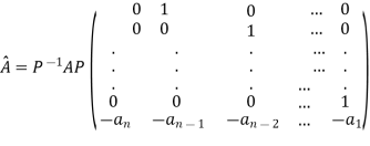
The model matrix is given as V= 
The above matrix is called as Vander Monde Matrix.
Examples
Q1) Find the eigenvectors of the matrix A= 
Sol: For eigenvalues | iI-A|=0
| I-A|=
I-A|= -
-  =0
=0
| I-A| =
  =0
=0
| I-A| = (
 +3)2-1=0
| I-A| =
 2+6
2+6 +8=0
+8=0
 1=-2,
1=-2,  2=-4
2=-4
For  1=-2 the eigenvectors are
 -
-  x Xi=0
 -
-  x
x  = 0
= 0

 = 0
= 0
-x1+x2=0
For x1=1 x2=1 the equation above is satisfied.
Xi=
For  2=-4
2=-4
 -
-  x
x  = 0
= 0

 = 0
= 0
-x1-x2=0
For x1=1 x2= -1 the equation above is satisfied.
Xi=
Q2) For the given matrix A=
Sol: For eigen values
| I-A|=
I-A|= -
-  =0
=0
| I-A| =
  =0
=0
| I-A| = (
 -3) (
-3) ( -2)-2=0
| I-A| =
 2-5
2-5 +4=0
+4=0
 1=1,
1=1,  2=4
2=4
For  1=1 the eigenvectors are
 -
-  x Xi=0
 -
-  x
x  = 0
= 0

 = 0
= 0
-2x1+2x2=0
For x1=1 x2=1 the equation above is satisfied.
X1=
For  2=4
2=4
 -
-  x
x  = 0
= 0

 = 0
= 0
x1+2x2=0
For x1=2 x2= -1 the equation above is satisfied.
X2=
Arrange eigenvectors in a matrix P = 
P-1= -  =
=
The transformation matrix  =P-1AP
=
=
=
Stability
The concept of stability can be understood by the following example.
Q) A system is represented by the state equation and output equation as
 =
=  +
+ u(t) and Y= [1 2]
Find the poles of the system and comment on stability?
Sol: A= 
The characteristic equation is given as
| I-A|=
I-A|= -
-  =0
=0
| I-A| =
  =0
=0
| I-A| = (
 +3) (
+3) ( +2)-2=0
| I-A| =
 2+5
2+5 +4=0
+4=0
 1=-1,
1=-1,  2=-4
2=-4
The poles are -1 and -4. Both on left half of s-plane so system is stable.
Controllability: A control system is said to be completely controllable if it’s possible to transfer the state of system from initial state to any other required state.
[S]= [B AB AB2 AB3 ------------------- An-1B]
Kalman’s Test: A system is said to be completely controllable if determinant of matrix is not equal to zero, or the rank of the following matrix should be to ‘n’.
n---- order of the matrix.
If  ≠0 then completely controllable
If  =0 then not controllable
Question: A system is represented by following state model A=  B=
B= find whether it is controllable or not?
Solution: A=  B=
B=
So, order of matrix is n=2
[S]= [B AB]
= 
 =0 hence, system is not controllable.
Observability: A system is said to be completely observable if it is possible to determine the initial state of system by observing the output for finite interval of time.
Calman’s Test: A system is said to be completely observable within the determinant of following matrix is not equal to zero, or, the matrix rank should be equal to 1.
[Q]= [CT ATCT (AT)2CT ----------(AT)n-1CT]
If ≠0 then completely observable
=0 then not observable
Question: A system is represented by following state model A=  B=
B= , C= [1 1] test whether the system is observable or not?
Solution: AT=  CT=
CT=
[Q]= [CT ATCT]
=

=

=
=0
 =0 hence not observable.
The state-space design method is based on the pole-placement method and the quadratic optimal regulator method. The pole placement method is similar to the root-locus method. In that we place closed-loop poles at desired locations. The basic difference is that in the root-locus design we place only the dominant closed loop poles at the desired locations, while in the pole-placement method we place all closed-loop poles at desired locations. The state variable feedback may be used to achieve the desired pole locations of the closed-loop transfer function. The approach is based on the feedback of all the state variables, and therefore u = Kx. When using this state variable feedback, the roots of the characteristic equation are placed where the transient performance meets the desired response.
The nth order state model is given as
 =Ax(t)+Bu(t)
y=Cx
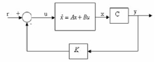
Fig: State variable feedback system
The state variable feedback is given as
 =Kx = [k1 k2 ……….kn]
The block diagram is shown above. From above figure we can write
u = -Kx+r
Where u = Plant input and r = system input
The necessary condition for pole placement is that the system should be completely controllable.
Design steps of pole placement:
- Check the controllability condition for the system. If system is completely controllable then proceed to next step.
- Determine a1, a2 …. an from matrix A using characteristic equation |
 I-A|= sn+a1sn-1+…...+an-1s+an
 - Determine transformation matrix T. By T=QW
Where Q=controllability matrix
W=
4. From the eigenvalues  …….
……. determine the characteristic polynomial (s-
 )(s-
)(s- )….(s-
 )= sn+α1sn-1+…..+ α n-1s+ αn. Then determine α1, α2,……. αn
5. Determine the state feedback matrix K, which is given as
K= [ αn- an αn-1 an-1 …………. α2 – a2 α1- a1] T-1
Just as with continuous-time control, we can choose to utilize a transfer function approach or a state variable approach to control. In this chapter we will utilize the transfer function approach, while in the remainder of these notes we will utilize the state variable approach. In this brief chapter we first discuss implementing discrete-time transfer functions, then talk about some common conventions used in control system.
Just as in continuous-time we will represent signals in either the time domain or the transform domain, which in this case is the z-transform domain. A simple input-output transfer function block is shown in Figure. While in the continuous time-domain it might be somewhat difficult to solve for the output in terms of the input in the time-domain, in the discrete-time domain we can just use the recursive relationship from the transfer function. Specifically, if we have the transfer function G(z), then we can write it as

Where n ≥ m. Converting this to the time domain, the output y(k) can be written in terms of previous output values and the current and previous input values as
y(k) = −a1y(k − 1) − a2y(k − 2) + · · · − any(k − n) + b0u(k) + b1u(k − 1) + ... + bmu(k − m)

Fig 3 Discrete-time transfer function
This is an Infinite Impulse Response (IIR) filter, since the output at any time depends on both previous outputs and previous inputs. If the output depended only on previous inputs, it would be a Finite Impulse Response (FIR) filter.
Nth order differential equation and transfer function
The phase variables are defined as the state variables obtained from any one of the system variables and its derivatives. The nth order linear differential equation for given input y(t) and output u(t) is given as
y(n)+a1y(n-1)+………..+an-1 +any=bou(m)+……+bm-1
 + bm u. ….. (9)
The initial conditions are expressed as y(0), ,…..,y(n-1)(0).
The transfer function assuming all initial conditions zero is
T(s)= = [b0sm+b1sm-1+…. +bm-1s+bm/ [sn+a1sn-1+……. +an-1s+an] …… (10)
Considering simple case when there are no zeros in the system, the transfer function becomes
T(s)= =[b]/ [sn+a1sn-1+……..+an-1s+an] …….(11)
For above transfer function the differential equation is given as
y(n)+a1y(n-1)+………..+an-1 +any=b u …….(12)
Let x1=y
x2=
…….
xn=y(n-1)
From (12) the differential equation is given as


……….

 =-anx1-an-1x2-…….-a1xn+bu

 =Ax+Bu ……….(13)
Note: Matrix A is known as Bush form or companion form. Matrix B has all elements zero except the last element.
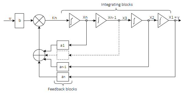
The output equation is given as y=x1
y=Cx ……….(14)
Where C = [1 0 0………..0]
State Equations of Sampled Data Systems
Let us assume that the following continuous time system is subject to sampling process with an interval of T
 =Ax(t) + Bu(t)
The above equation is the state equation
y(t) = Cx(t) +Du(t)
The above equation is the output equation.
We know that the solution to above state equation is

Since the inputs are constants in between two sampling instants, one can write:

Which implies that the following expression is valid within the interval kT ≤ τ ≤ (k + 1) T if we consider t0 = kT

Let us denote

Then we can write

If t = (k + 1) T,

Where

If t ′ = τ − kT, we can rewrite θ(T) as

If we consider φ(T) = A¯ and θ(T) = B¯. Similarly, by setting t = kT, one can show that the output equation also has a similar form as that of the continuous time one.
When T = 1,


State Equations of Inherently Discrete Systems
When a discrete system is composed of all digital signals, the state and output equations can be described by
x (k + 1) = Ax(k) + Bu(k)
y(k) = Cx(k) + Du(k)
Discrete Time Approximation of Continuous Time State Space Model
Let us consider the dynamical system described by the state space mode. By approximating the derivative at t = kT using forward difference, we can write:


And


If T=1


We can thus conclude from the discussions so far that the discrete time state variable model of a system can be described by
x (k + 1) = Ax(k) + Bu(k)
y(k) = Cx(k) + Du(k)
Where A, B are either the descriptions of an all-digital system or obtained by sampling the continuous time process.
Stability is the most important issue in control system design. Before discussing the stability test let us first introduce the following notions of stability for a linear time invariant (LTI) system.
1. BIBO stability or zero state stability
2. Internal stability or zero input stability
Since we have not introduced the concept of state variables yet, as of now, we will limit our discussion to BIBO stability only. An initially relaxed (all the initial conditions of the system are zero) LTI system is said to be BIBO stable if for every bounded input, the output is also bounded. However, the stability of the following closed loop system
C(z)/R(z) =G(z)/1+GH
Can be determined from the location of closed loop poles in z-plane which are the roots of the characteristic equation
1 + GH(z) = 0
1. For the system to be stable, the closed loop poles or the roots of the characteristic equation must lie within the unit circle in z-plane. Otherwise, the system would be unstable.
2. If a simple pole lies at |z| = 1, the system becomes marginally stable. Similarly, if a pair of complex conjugate poles lie on the |z| = 1 circle, the system is marginally stable. Multiple poles on unit circle make the system unstable.
Example
Q1) Determine the closed loop stability of the system shown in Figure when K = 1

A)

Since it is unity feedback system, we have H(z)=1


We know that the characteristics equation is
1 + G(z) = 0
(z − 1) (z − 0.368) + 0.368z + 0.264 = 0
z2 − z + 0.632 = 0
z1 = 0.5 + 0.618j
z2 = 0.5 − 0.618j
Since |z1| = |z2| < 1, the system is stable.
Three stability tests can be applied directly to the characteristic equation without solving for the roots.
- Schur-Cohn stability test
- Jury Stability test
- Routh stability coupled with bi-linear transformation.
Computation requirements in Jury test is simpler than Schur Cohn when the co-efficient are real which is always true for physical systems.
Jury Stability Test
Assume that the characteristic equation is as follows,
P(z) = a0zn + a1z n−1 + ... + an−1z + an
Where a0 > 0.
Jury Table
 |  |  |  | … | … |  |
 |  |  |  | … | … |  |
 |  |  |  | … | … |  |
 |  |  |  | … | … |  |
 |  |  |  | … | … |  |
 |  |  |  | … | … |  |
 |  |  |  | … | … |  |
. . . | ... ... ... | ... ... ... | ... ... ... | ... ... ... | ... ... ... | ... ... ... |
 |  |  |  |
|
|
|

k = 0, 1, 2, 3, ...., n – 1

k = 0, 1, 2, 3, ...., n – 2

This system will be stable if
1. |an| < a0
2. P(z)|z=1 > 0
3. P(z)|z=−1 > 0 for n even and P(z)|z=−1 < 0 for n odd
4.


. …….
. …….

Q2) The characteristic equation: P(z) = z4 − 1.2z3 + 0.07z2 + 0.3z − 0.08 = 0 Thus, a0 = 1, a1 = −1.2, a2 = 0.07, a3 = 0.3, a4 = −0.08. By Jury test comment on stability.
A2) We will now check the stability conditions.
1. |an| = |a4| = 0.08 < a0 = 1 ⇒ First condition is satisfied.
2. P (1) = 1 − 1.2 + 0.07 + 0.3 − 0.08 = 0.09 > 0
Second condition is satisfied.
3. P (−1) = 1 + 1.2 + 0.07 − 0.3 − 0.08 = 1.89 > 0
Third condition is satisfied
Jury Table

= 0.0064 − 1 = −0.9936

= −0.08 × 0.3 + 1.2 = 1.176
Rest of the elements are also calculated in a similar fashion.
The elements are b1 = −0.0756
b0 = −0.204
c2 = 0.946
c1 = −1.184
c0 = 0.315.
One can see |b3| = 0.9936 > |b0| = 0.204 |c2| = 0.946 > |c0| = 0.315
All criteria are satisfied. Thus, the system is stable.
Q3) The characteristic equation: P(z) = z3 − 1.3z2 − 0.08z + 0.24 = 0 Thus a0 = 1, a1 = −1.3, a2 = −0.08, a3 = 0.24. Comment on stability.
A3) Stability conditions are:
- |a3| = 0.24 < a0 = 1 so First condition is satisfied.
- P (1) = 1 − 1.3 − 0.08 + 0.24 = −0.14 < 0. The Second condition is not satisfied.
Since one of the criteria is violated, we may stop the test here and conclude that the system is unstable. P (1) = 0 or P (−1) = 0 indicates the presence of a root on the unit circle and in that case the system can at the most become marginally stable if rest of the conditions are satisfied.
Q4) Consider the system shown in Figure. Find out the range of K for which the system is stable.

A4)

The closed loop transfer function

Characteristic equation: P(z) = z2 + (0.368K − 1.368) z + 0.368 + 0.264K = 0
Since it is a second order system only 3 stability conditions will be there.
1. |a2| < a0
2. P (1) > 0 3. P (−1) > 0 since n = 2=even. This implies:
1. |0.368 + 0.264K| < 1
2.39 > K > −5.18
2. P (1) = 1 + (0.368K − 1.368) + 0.368 + 0.264K = 0.632K > 0 ⇒ K > 0
3. P (−1) = 1 − (0.368K − 1.368) + 0.368 + 0.264K = 2.736 − 0.104K > 0 ⇒ 26.38 > K
Combining all, the range of K is found to be 0 < K < 2.39.
If K = 2.39, system becomes critically stable.
The characteristics equation becomes
z2 − 0.49z + 1 = 0
z = 0.244 ± j0.97
Sampling period T = 1 sec.
wd = (ws/2π) ∠z = (2π/2π) tan−1 (0.97/0.244) = 1.324 rad/sec
The above frequency is the frequency of sustained oscillation.
Ii) Bilinear Transformation:
In z-domain for the system to be stable the roots of the characteristic equation must lie within the unit circle. But the transform z=esT cannot be used because the periodicity of esT and multiple strips of left half of s-plane into which the interior of the unit circle maps.
The Bilinear transformation maps the interior of the unit circle in the z-plane into the left half of r-plane.
r=
z=
On the unit circle in the z-plane
z=

r= =
= =tanhj
 =jtan
=jtan =j
=j r
r
 r= tan
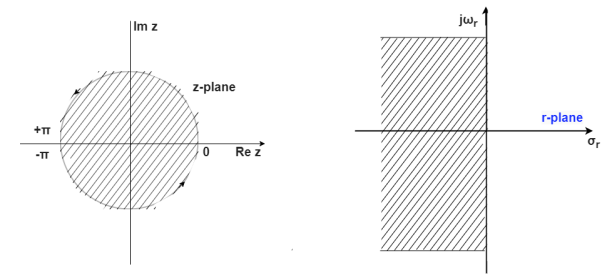
The characteristic equation is
an + an-1
  +………...+a1
 +a0=0
+a0=0
Q) Using bilinear transformation determine the characteristic equation of given open loop function in z-plane. G(s)=
Sol: G(s)=
=5[  ]
]
=5[  ]
]
=
The characteristic equation is given as
1+G(S)= +
+ =0
=0
z3-0.5z2+2.49z-0.496=0
Putting in equation below
The characteristic equation is
an + an-1
  +………...+a1
 +a0=0
+a0=0
 -0.5
-0.5 +2.49
+2.49 -0.496=0
3.5r3-2.5r2+0.5r+2.5=0
The system stability can be checked using Routh array
The characteristic equation in s-domain will be
1+G(s)=0
1+ =0
=0
s3+3s2+2s+5=0
s3 1 2
s2 3 5
s1 1/3 0
s0 5 0
First column no sign change. Hence, system is stable.
Singular Cases
When some or all of the elements of a row in the Jury table are zero, the tabulation ends prematurely. This situation is referred to as a singular case. It can be avoided by expanding or contracting unit circle infinitesimally by an amount  which is equivalent to move the roots of P(z) off the unit circle.
The transformation is
z1 = (1 +  )z
)z
Where  is a very small number. When
  is positive the unit circle is expanded and when
  is negative the unit circle is contracted. The difference between the number of zeros found inside or outside the unit circle when the unit circle is expanded or contracted is the number of zeros on the unit circle. Since (1 +
  )n zn ∼= (1 + n
 )zn for both positive and negative
  , the transformation requires the coefficient of the zn term be multiplied by (1 + n
 ).
).
Q5) The characteristic equation: P(z) = z3 + 0.25z2 + z + 0.25 = 0 Thus, a0 = 1, a1 = 0.25, a2 = 1, a3 = 0.25. Comment on stability?
A5) We will now check the stability conditions.
1. |an| = |a3| = 0.25 < a0 = 1
First condition is satisfied.
2. P (1) = 1 + 0.25 + 1 + 0.25 = 2.5 > 0
Second condition is satisfied.
3. P (−1) = −1 + 0.25 − 1 + 0.25 = −1.5 < 0
Third condition is satisfied.
Jury Table


Thus, the tabulation ends here and we know that some of the roots lie on the unit circle. If we replace z by (1 +  )z,
)z,
The characteristic equation would become
(1 + 3 )z 3 + 0.25(1 + 2
 )z 2 + (1 +
  )z + 0.25 = 0
First three stability conditions are satisfied.
 |  |  |  |  |
 | 0.25 | 1+ | 0.25(1+2) | 1+3 |
 | 1+3 | 0.25(1+2) | 1+ | 0.25 |
 |  |   |  |
|
|b2| = |0.0625 − (1 + 6 + 9
+ 9 2 )| and |b0| = |1 + 3.875
 + 3
+ 3 2 − 0.0625|. Since, when
  → 0 +,
1 + 6 + 9
+ 9 2 > 1 + 3.875
 + 3
+ 3 2, thus |b2| > |b0| which implies that the roots which are not on the unit circle are actually inside it and the system is marginally stable.
References:
[1] I. J. Nagrath and M. Gopal, “Control Systems Engineering”, New Age International,
2009.
[2] K. Ogata, “Modern Control Engineering”, Prentice Hall, 1991
[3] M. Gopal, “Control Systems: Principles and Design”, McGraw Hill Education, 1997.