Unit - 2

Production, Cost and Revenue Concepts

2.1 Production: Production function, Laws of returns: Law of variable proportion, Law of returns to scale

Meaning of production:

Since the main purpose of economic activity is to generate benefits for the individual, we count as production during a period of time all activities that either generate benefits during the period or increase the ability of society to generate benefits in the future.

Companies are important components (units) of the economic system

They are artificial units created by individuals to organize and facilitate production.

The essential characteristic of the company is that it purchases factors of production such as land, labor, capital, intermediate products and raw materials from households and other businesses and converts these resources into various goods or services that it sells to its customers. Other commercial enterprises and various government units as well as abroad.

Definition of production:

According to Bates and Parkinson:

“Production is the organized activity of converting resources into finished products in the form of goods and services. The aim of production is to meet the demand for such transformed resources”.

According to J. R. Hicks:

Production is any interest those pursuits to fulfil the wishes of different humans via exchange. This definition makes it clean that during enterprise we do now no longer deal with the mere making of factors as manufacturing. What is finished should be designed in one of these manners that it satisfies the wishes.

For general purposes, it is necessary to classify production into three main groups:

1. Primary production:

Primary production is carried out by raw material industries such as agriculture and forestry, fishing, mining and oil production. Among other things, these industries are engaged in extracting the gifts of nature from the surface, below the surface and from the oceans.

2. Secondary production:

This includes production in the manufacturing industry, namely the manufacture of semi-finished and finished goods from raw materials and intermediate products - converting flour into bread or iron ore into finished steel. They are commonly referred to as the manufacturing and construction industries, such as the manufacture of automobiles, furnishings, clothing and chemicals, and engineering and construction.

3. Tertiary production:

Industries with inside the tertiary area offer all of the offerings that allow the completed items to be located with inside the arms of the consumer. In fact, those offerings are introduced to corporations in all industries and at once to consumers. Examples are retailers, banks, coverage companies, transportation and communications. Government offerings which include regulation, administration, education, health, and defence also are included.

Production function

To have clear knowledge about production and cost it’s mandatory to know the basics of production functions and understand the fundamentals in mathematical terms. We break down short-term and long-term production functions supported variable and glued factors.

What is the production function?

The purposeful courting among the bodily enter (or aspect of manufacturing) and consequently the output is called a manufacturing characteristic. It assumed the enter as an explanatory or unbiased variable and the output as an established variable.

Mathematically, you can write this as:

Q=f (L, K)

Where Q represents the output; “L” and “K” are the inputs, respectively, labour and capital (inclusive of machinery). Note that there can be many different elements, however we're assuming a -aspect enter here. Production capabilities are described in another way withinside the quick time period and withinside the lengthy time period. This difference is critical in microeconomics. This difference is primarily based totally on the character of the aspect enter.

Inputs that extrade at once with the output are known as variable elements. These are elements that may extrade. Fluctuating elements exist each withinside the quick time period and withinside the lengthy time period. Examples of variable elements encompass day by day labour and uncooked materials.

On the opposite hand, elements that cannot extrade or extrade because the output modifications are known as constant elements. These elements are typically function best for a quick or quick duration of time. There aren't any constant elements withinside the lengthy time period.

Therefore, manufacturing capabilities may be described: quick-time period and lengthy-time period. A quick-time period manufacturing characteristic defines the relationship among one variable aspect (maintaining all different elements constant) and consequently the output. The regulation of regression to elements explains one of these manufacturing characteristics.

For instance, think that an agency has 20 gadgets of Labour and six acres of land, and to begin with makes use of best Labour gadgets (variable coefficients) for that land (constant coefficients). Thus, the ratio of land and labour is 6: 1. Now, if the agency chooses to undertake 2 labour gadgets, then the ratio of land to Labour could be 3: 1 (6: 2). Here, all elements extrade withinside the identical share. The regulation used to give an explanation for that is known as the regulation of go back to scale. It measures how a lot of the output modifications while the enter modifications proportionally.

Laws of returns: Law of variable proportion, Law of returns to scale

Law of variable proportion

The regulation of variable proportions or the go back to elements performs an essential position with inside the have a take a observe of the concept of manufacturing. In this article, we are able to study the meanings, explanations, ranges, significance, and motives at the back of the operation of the regulation of variable proportions.    

Law of variable proportions or factor of a variable

This law indicates a short-term production function in which one factor changes and the other is fixed.

Also, if you get an extra output when applying an extra unit of input, this output will be equal to or less than the output obtained from the previous unit.

The law of variable proportions relates to how the output changes when the number of units of variable factors is increased. Thus, it refers to the effect of the changing factor ratio on the output.

In other words, this law shows the relationship between the unit of variable factors and the volume of production in the short term. This assumes that all other factors are constant. This relationship is also known as the return to variable factors.

The law states that if we keep other factors constant, then when we increase the variable factor, the total product first increases at the rate of increase, then at the rate of decrease, and finally begins to decrease. Why is it called the law of variable proportions?

The factor ratio or factor ratio changes because one input changes and everything else remains constant. Let's take an example to better understand this:

Let's say you have 10 acres of land and 1 unit of labour for production. So, the ratio of land and labour is 10: 1. Now, if we increase the unit of Labour to 2 while keeping the land constant, then the ratio of land to Labour will be 5: 1.

Thus, as you can see, the law analyses the effect of changes in the factor ratio on the amount of out, and hence is called the law of variable proportions.

The law of proportion of variables explained

Let's understand this law with the help of another example:

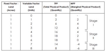
In this example, land is a fixed factor and labour is a variable factor.

The following figure describes the law of variable proportions. For a simple representation, the total physical product (TPP) curve and the limit physical product (MPP) curve are drawn as smooth curves for variable inputs (labour). Three stages of law

The law has three stages:

Stage I–TPP will increase at an increasing rate, and MPP will increase too. The MPP increases with the increase of the variable factor unit. Therefore, it's also called the stage of accelerating returns. In this example, Phase I of the law runs up to three units of labour (between points O and L).

Stage II–TPP continues to increase, but is declining. But the increase is a plus. In addition, the MPP decreases with an increase in the number of units of the variable factor. Therefore, it is called the stage of Return of decline. In this example, Stage II is performed between four to six units of labour (between points L and M). This stage reaches the point where TPP is maximum (18 in the example above) and MPP is zero (point R).

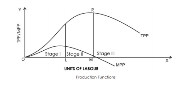
Stage III- now the TPP begins to decrease, the MPP decreases and goes to the negative. Therefore, it's called the stage of negative returns. In this example, Stage III is performed between seven and eight units of labour (from Point M onwards).

Significance of three stages

Stage I

At this stage, the marginal product increases with an increase in the variable factor.

Thus, producers can adopt more units of variables to efficiently utilize fixed factors. So, the producers would prefer not to stop at stage I, but try to expand further.

Stage II

Producers do not like to work even in Stage III. At this stage, there is a decrease in the total product, and the marginal product becomes negative.

To increase output, producers reduce the amount of variable factors. However, in Stage III, the cost of generating an increase will be less profitable and the profit will decrease.

Stage III

Any intelligent producer avoids the first as well as the third stage of production. Therefore, producers prefer Stage II–a stage that reduces returns. This stage is the most relevant stage of operation for producers, according to the law of variable proportions.

The law of variable proportions in terms of TPP and MPP

The description is as follows:

The law of the rate of change-from the perspective of the TPP

We know that the law of variable proportions shows the relationship between the units of variable factors and the total physical product.

Also, if you keep other factors constant and increase the unit of variable factors, the TPP will initially increase at the rate of increase, then decrease, and eventually decrease. So, there are three distinct stages:

I-TPP is increasing at an increasing rate

II-TPP is increasing at a declining rate

III-TPP decline

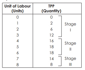
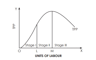
Example of the law of variable ratios from the point of view of MPP and from the point of view of TPP Law

I-MPP increase

II-MPP decreases, but remains positive

III-MPP continues to decrease and becomes negative

Reasons for the operation of the law

In the short term, we cannot change all the factors of production.

In this case, there is only one variable factor, and the other is fixed.

All other factors combine optimally to produce maximum output.

Thus, the marginal physical product increases.

In the early stages, when producers adopt more units of variable factor versus fixed factor, the total product tends to rise at an increasing rate.

Then, beyond the point of optimal combination, if the producer adopts more units of variable factors, the factor proportion becomes inefficient. Thus, the marginal product of its variable factor decreases.

Also, producers see that as they increase the unit of variable factors, the amount of fixed factor input per unit of variable decreases.

Therefore, successive units of variable inputs add the reduced amount to the total output because there are fewer fixed inputs to operate.

Law of returns to scale

In the long run, all factors of production will fluctuate. The factor is not fixed.

Therefore, the dimensions of manufacturing may be modified through converting the amount of all elements of manufacturing.

Meaning:

"The term scale harvest refers to changes in production when all factors change at the same rate." Koutsoyiannis

"The harvest on scale is a long-term concept, related to the behavior of total output when all inputs change." Rybavsky

There are three types of scale harvests:

1. Increasing returns on scale.

2. Harvest on a certain scale

3. Diminishing returns on scale

Explanation:

In the long run, you can increase the output by increasing all the factors at the same rate. In general, the law of harvest regarding scale refers to an increase in production due to an increase in all factors at the same rate. Such an increase is called a scale harvest.

Suppose your first production function looks like this:

P = f (L, K)

Now, if the factor of production, that is, both labor and capital, increases at the same rate, that is, x, then the product function is rewritten as:

1. If increases in the same proportion as the increase in factors of production i.e., , it will be constant returns to scale.

2. If increases less than proportionate increase in the factors of production i.e., , it will be diminishing returns to scale.

3. If increases more than proportionate increase in the factors of production i.e., , it will be increasing returns to scale.

Returns to scale can be shown with the help of table 8.

Table 8 Showing different stages of return to scale

The table above describes the following three stages of harvesting in terms of scale.

1. Increasing returns on scale:

Increasing returns or reducing costs in terms of scale refers to a situation in which all factors of production increase and production increases at a higher rate. That is, when all inputs are doubled, so is the output, which increases faster than double. Therefore, it is said to be increasing returns in terms of scale. This increase is due to a number of reasons, including the sector's external economies of scale. Increasing returns in terms of scale can be explained with the help of Figure 8.

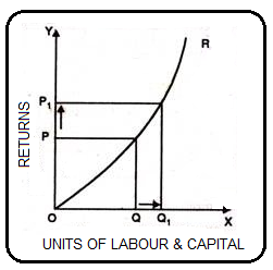
In Figure, the OX axis represents the increase in labour and capital, and the OY axis represents the increase in production. As labour and capital increase from Q to Q1, the factor of production also increases from P to P1. This is higher than the factor of production: labour and capital.

2. Diminishing returns on scale:

Diminishing returns or increased costs refer to a production situation in which production increases at a lower rate if all elements of production increase at a certain rate. That is, if the input is doubled, the output is less than doubled. An example of diminishing returns in terms of scale is when production increases by 10% after a 20% increase in labour and capital.

The main cause of diminishing returns operations in terms of scale is that the internal and external economies are less than the internal and external uneconomic. This is clear from Figure 9.

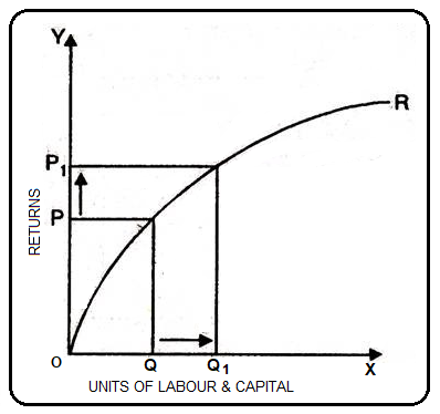
This Figure shows diminishing returns in terms of scale. The OX axis gives labor and capital, and the OY axis gives output. If the factor of production increases from Q to Q1 (more quantity), but as a result the production increases, that is, P to P1 decreases. We can see that diminishing returns in terms of scale apply because the factor of production increases more and the increase in production is relatively small.

3. Harvest on a certain scale:

A harvest or a constant cost on a certain scale is a production situation in which production increases at exactly the same rate as the factor of production increases. Simply put, when the factor of production doubles, so does the production.

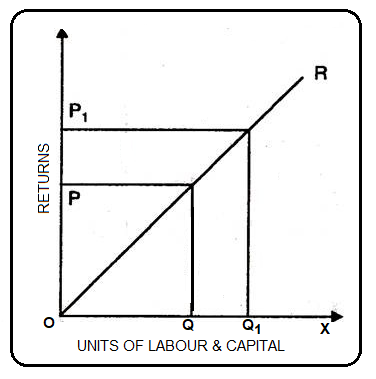
In this case, the internal and external economies are exactly the same as the internal and external economies. This situation occurs when economies of scale and economies of scale are balanced after reaching a certain production level. This is known as the homogeneous production function. The Cobb-Douglas linear homogeneous production function is a good example of this kind. This is shown in Figure. In Figure, we can see that the factor of production, that is, the increase in labor and capital, is equal to the rate of increase in the factor of production. Therefore, the result is a harvest on a certain scale.

Key takeaways:

1. Companies are important components (units) of the economic system
2. “Production is the organized activity of converting resources into finished products in the form of goods and services. The aim of production is to meet the demand for such transformed resources”.
3. Primary production is carried out by raw material industries such as agriculture and forestry, fishing, mining and oil production.
4. Industries in the tertiary sector provide all the services that enable the finished goods to be placed in the hands of the consumer.
5. The functional relationship between the physical input (or factor of production) and therefore the output is named a production function.
6. The law of variable proportions or the return to factors plays an important role in the study of the theory of production
7. The law of variable proportions has three stages.
8. Producers do not like to work even in Stage III. At this stage, there is a decrease in the total product, and the marginal product becomes negative.
9. Any intelligent producer avoids the first as well as the third stage of production.
10. Successive units of variable inputs add the reduced amount to the total output because there are fewer fixed inputs to operate.
11. In the long run, all factors of production will fluctuate. The factor is not fixed. Therefore, the scale of production can be changed by changing the quantity of all factors of production.
12. "The term scale harvest refers to changes in production when all factors change at the same rate."
13. Increasing returns or reducing costs in terms of scale refers to a situation in which all factors of production increase and production increases at a higher rate.
14. Diminishing returns or increased costs refer to a production situation in which production increases at a lower rate if all elements of production increase at a certain rate.

2.2 Cost and Revenue concepts: Total Cost, Fixed Cost, Variable Cost, Total Revenue, Average Revenue and Marginal Revenue, Cost – Output Relationships in the Short Run, Cost – Output Relationships in the Long Run, Analysis of cost minimizations   

Total Cost:

Total cost(TC) refers to the sum of fixed and variable costs incurred in the short term. So, the short-term cost can be expressed as follows

TC=TFC+TVC

Note that in the long run, TFC=0, so TC = TVC. So you can get the shape of the TC curve by summing the TFC curve and the TVC curve.

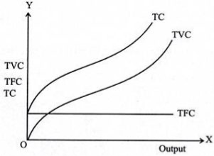
For the TC curve, the following points can be noted:

• The TC curve is shaped of reverse S. This is because of the TVC curve. Since the TFC curve is horizontal, the difference between the TC curve and the TVC curve is the same at each level of the output and is equal to the tfc. This is explained as follows: TC-TVC=TFC
• The TFC curve is parallel to the horizontal axis, and the TVC curve is inverted S-shaped.
• The law that explains the Shape of TVC and subsequent TC is called the law of variable proportions.

Fixed Cost:

1. Fixed cost (TFC)-

1. Fixed cost remains fixed in short run period. The cost does not change with the change in the level of output.
2. These costs are also called indirect costs, overhead costs, historical costs, and unavoidable costs.

c.   Definition

1. In the words of Ferguson, “Fixed cost is the sum of the ‘short run explicit fixed costs and implicit costs incurred by the entrepreneur.”

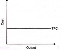
b.  From the above figure, we can see TFC curve is horizontal to X axis. TFC remains constant with proportionate change in the output.

Variable Cost

1. Refers to the cost changes with the change in the level of output.
2. Ex – cost incurred in purchase of raw material, hiring labour, etc
3. Definition

According to Ferguson, “Variable cost is the sum of amounts spent for each of the variable inputs used”

1. If the output is zero, variable cost is zero.
2. These costs are also called prime costs, direct costs, and avoidable costs.

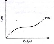
In the above figure, TVC changes with the change in the level of production.

Total Revenue

Gross sales, additionally called gross sales, refers to the entire sales generated via way of means of an organisation from all income of products or offerings. For example, if you run an ice cream shop, your total revenue includes sales of all ice cream, not just sales from one flavor or type of Sunday.

Determining a company's total revenue can be a useful determinant in assessing a company's financial position. The higher your total income, the more money your company is making. This is especially useful if you have a lot of money to cover. A high total income means that you have enough income to cover these costs and that you have the means to maintain ups and downs and profits for the foreseeable future.

How to calculate total income

The better you understand your total revenue, the more accurate your calculations will be. An easy way to calculate your company's total revenue is to first determine the total number of units your company has sold and the average price per unit sold. Total revenue depends on these two values. Then, to determine your total revenue, simply multiply the number of units sold by the average price per item. You also need to add interest or dividends to determine your total income.

Use the following formula when calculating your company's total revenue.

Gross income = (average price per unit sold) x (unit sales)

For service-based businesses, replace the average price per unit with the average price per service sold and the number of units sold with the number of services sold. For example:

Total revenue = (average price per service sold) x (number of services sold)

The value obtained from these calculations is total revenue. Make sure you take into account the financial changes in your company's finances, no matter how big or small.

For example, if you change the price of a unit or service sold, you should consider this change as it can distort your calculations. Also, be sure to include non-operating income such as investment income and dividend income in the calculation.

Average Revenue and Marginal Revenue

Average sales refer back to the sales earned via way of means of a vendor via way of means of promoting a unit product. This is received via way of means of dividing the entire earnings via way of means of the entire manufacturing. “The common sales curve indicates that the charges of the organisation's merchandise are the identical at every manufacturing degree.” Stonier and the Hague

Thus:

Where Average Revenue; TR=Total Revenue; Q= output

According to McDonnell “Average Revenue is the per unit revenue received from the sale of one unit of commoditiy.”

TR=Price × Output

TR=Pq

And P=f(Q) is an average curve which shows that price is a function of quantity demanded. It is also a demand curve.

Marginal sales is the internet sales earned via way of means of promoting extra devices of a product. “Marginal sales is the alternate in general sales that consequences from the sale of 1 greater or one much less unit of manufacturing.” Ferguson.

Therefore, marginal revenue is delivered to general sales via way of means of promoting some other unit of products. Algebraically, marginal sales is the internet addition to general sales from promoting n devices of products in preference to n – 1.

Therefore, A. Koutsoyiannis, “The marginal revenue is the alternate in general sales due to promoting a further unit of the commodity.”

Therefore,

Whereas

Marginal revenue from nth unit

n= Any given number

If total revenue from (n) units is 110 and from (n – 1) units is 100.in that case

MRnth = TRn – TRn _ 1 = 100 – 100

MRnth = 10

MR in mathematical terms is the ratio of change in total revenue to change in output

MR = ∆TR/∆q or dR/dq = MR

The relation of total revenue, average revenue and marginal revenue can be explained with the help of table and fig.

Table Representation:

The relationship between TR, AR and MR can be expressed with the help of a table.

Unit (q)	TR/q AR or Price	(Pq) TR	(T
1 2 3 4 5 6 7 8 9 10	10 9 8 7 6 5 4 3 2 1	10 18 24 28 30 30 28 24 18 10	10 8 6 4 2 0 -2 -4 -6 -8

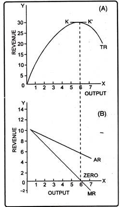
From the table, we can draw the idea that as the price falls from Rs. 10 to Re. 1, the output sold increases from 1 to 10. Total revenue increases from 10 to 30, at 5 units. However, at 6th unit it becomes constant and ultimately starts falling at next unit i.e., 7th. In the same way, when AR falls, MR falls more and becomes zero at 6th unit and then negative. Therefore, it is clear that when AR falls, MR also falls more than that of AR: TR increases initially at a diminishing rate, it reaches maximum and then starts falling.

The formula to calculate TR, AR and MR is as under:

TR = P x q

Or TR = MR1 + MR2 + MR3 + MR3 +…... MR„

TR

AR = TR/q MR = TRn – TRn _ x

In fig. 1 three concepts of revenue have been explained. The units of output have been shown on horizontal axis while revenue on vertical axis. Here TR, AR, MR are total revenue, average revenue and marginal revenue curves respectively.

In figure 1 (A), a total revenue curve is sloping upward from the origin to point K. From point K to K’ total revenue is constant. But at point K’ total revenue is maximum and begins to fall. It means even by selling more unit’s total revenue is falling. In such a situation, marginal revenue becomes negative.

Similarly, in the figure 1 (B) average revenue curves are sloping downward. It means average revenue falls as more and more units are sold.

In fig. 1 (B) MR is the marginal revenue curve which slopes downward. It signifies the fact that MR with the sale of every additional unit tends to diminish. Moreover, it is also clear from the fig. That when both AR and MR are falling, MR is less than AR. MR can be zero, positive or negative but AR is always positive.

Cost – Output Relationships in the Short Run

For research on the relationship between cost and output. There are two aspects: the short-term cost-output relationship and

2. The long-term cost-output relationship.

The short term is the period during which fixed equipment (machinery, buildings, etc.) and organizational changes are not permitted. Therefore, if you need to increase production, you can do so within the limits allowed by existing fixed factors of production.

In the long run, there is enough time to resize equipment (machinery, buildings, land, etc.) and organizations. In this way, in the long run, the factors of production themselves can be changed, allowing you to increase production without being limited by fixed factors of production.

i.    Average fixed cost output:

The higher the output, the lower the fixed cost per unit, or average fixed cost. The cause is that general constant prices continue to be the identical and do now no longer alternate with adjustments in manufacturing. The relationship between output and fixed costs is universal for all types of businesses.

Therefore, average fixed costs continue to decline as production increases. The reason the total fixed costs remain the same and the average fixed costs decrease is that certain factors are inseparable. Indivisible means that if you produce less output, you cannot use that coefficient in a smaller amount. Use as a whole.

Ii.     Average variable cost and output:

As more units are produced in a particular plant, average variable costs fall first and then rise. This is because adding variable coefficient units to a fixed plant first increases the efficiency of the input and then decreases it. In fact, variable factors tend to generate somewhat more efficiently near the enterprise's optimal output than at very low levels of output.

However, when the optimum capacity is reached, the average variable cost will undoubtedly increase significantly as the output increases further. You can get more output, but the average variable cost is much higher. For example, if more and more workers are appointed. It can eventually lead to overcrowding and bad organization. In addition, workers may have to pay higher wages for overtime.

Iii.    Average total cost and output:

The average total cost, more commonly known as the average cost, decreases first and then increases. The important point to note here is that the turning point for average costs is a bit behind for average variable costs.

The average cost consists of the average fixed cost and the average variable cost. As we have seen, average fixed costs continue to decline as production increases, while average variable costs decrease first and then rise. As long as the average variable cost decreases, so does the average total cost. However, after some point, the average variable cost will rise. Here, even if the increase in variable costs is less than the decrease in fixed costs, the average total cost will continue to decrease.

Only if the increase in average variable costs is greater than the decrease in average fixed costs will the average total cost increase. Therefore, the increase in average variable costs is smaller than the decrease in average fixed costs, so the average variable costs have begun to rise, but the average total cost is still declining. The net effect is a reduction in average cost.

Minimum Cost-The output level is the level that has the lowest average total cost and is not the average variable cost. In fact, at the lowest cost output level, the average variable cost is greater than its minimum (average variable cost). The lowest cost output level is also the optimum output level. It may not be the maximum output level. Companies may decide to produce more than the lowest cost output level.

Iv      Short-term output cost curve:

The relationship between cost and output can also be displayed using a graph. You can see that the average fixed cost curve (AFC curve) decreases as the output rises from a low level to a high level. Therefore, the shape of the average fixed cost curve is a rectangular hyperbola.

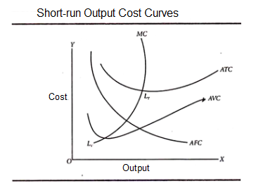
However, the average variable cost curve (AVC curve) begins to rise faster than the ATC curve. In addition, the minimum cost level of output corresponds to the point LT on the ATC curve, not the point LV on the AVC curve. Another important point is the marginal cost curve (MC curve) in Figure 3.2. It intersects both the AVC and ATC curves at the lowest point. This is very easy to explain. If the marginal cost (MC) is less than the average cost (AC), the AC will be reduced. If MC is greater than AC, raise AC. If MC is equal to AC, then AC is not raised or lowered. Therefore, the MC curve tends to intersect the AC curve at its lowest point.

Similarly, there is a view on the average variable cost curve. It makes no difference whether the MC is up or down. LT is the lowest total cost and LV is the lowest variable cost.

The interrelationships between AVC, ATC, and AFC can be summarized as follows:

1. If both AFC and AVC are reduced, so is ATC.

2. If AFC decreases but AVC increases:

(A) If the decrease in AFC is greater than the increase in AVC, the ATC will decrease.

(B) If the decrease in AFC is equal to the increase in AVC, the ATC will not decrease.

(C) If the decrease in AFC is less than the increase in AVC, the ATC will increase.

Cost – Output Relationships in the Long Run

Long-term cost:

To study the relationship between cost and output in the long run, we need to explain the concept of long-term cost.

In the long term, it is long enough to fluctuate all costs, including those that are fixed in the short term. In the short term, output fluctuations are only possible to the extent permitted by existing fixed plants and equipment. But in the long run, the entrepreneur has many options before him, including the construction of plants of various types and sizes.

Therefore, the company has enough time to fully adapt the plant, so there are no fixed costs. And all costs fluctuate. With this in mind, long-term cost refers to the cost of producing different levels of production due to changes in plant size or production scale. The relationship between long-term cost and output is graphed by a long-term cost curve (a curve that shows how costs change when production scale changes).

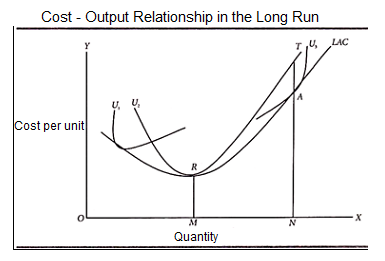
The concept of long-term costs can be further explained using illustrations. Suppose a company operates under the average total cost curve U2 at a particular time and generates an OM. Here, it is desirable to generate ON. If the company continues on an older scale, its average cost curve will be NT. If the company is resized, the new cost curve will be U3. In that case, the average cost to generate an ON would be NA.

NA is less than NT. Therefore, the new scale is preferable to the old scale and should be adopted. In the long run, the average cost to generate an ON output is NA. This is sometimes referred to as the long-term cost of producing an ON output. Note that we call it NA as a long-term cost only if the U3 scale is in the planning stage and is not actually adopted. The moment you install the scale, the NA cost becomes the short-term cost to generate the ON output.

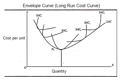
To draw a long-term cost curve, you need to start with some short-term average cost curves (SAC curves). Each such curve represents a particular scale or size of the plant, including the optimal scale. You can now draw a long-term cost curve that touches the entire family of SAC curves. That is, it touches each SAC curve at one point.

In this regard, you should be aware of the following:

1. The LAC curve touches various SAC curves. It is often referred to as the "envelope" because it is said to wrap them and the points on the SAC curve never fall below the LAC curve.

2. The LAC curve is like a U-shape or a "dish". The U-shape of the LAC curve means that the average cost will initially decrease and decrease until the optimal size of the enterprise is reached. After that, the average cost goes up continuously. That is, a plant larger than the optimal size is used.

The tendency for long-term average costs to decline as a company grows is a reflection of the cost economy as it grows, and the final rise in the long-term cost curve is primarily due to the final setting. In an uneconomical scale.

The SAC curve also has a U shape, with the difference that the LAC curve is flatter. In other words, the U-shape of the LAC curve is less noticeable. Such an economy is possible in the long run. Similarly, some of the uneconomic we face in the short term may not be faced in the long term.

3. The long-term average cost curve cannot cut the short-term average cost curve (although they are tangential to each other). This means that for a particular output, the average cost will not be higher in the long term than in the short term. This is because adjustments that reduce costs are possible in the short and long term. On the other hand, in the short term, it may not always be possible to produce a particular output in the cheapest way possible.

4. The LAC curve touches the "optimal scale" curve at the latter minimum cost point, N1.

5. The LAC curve touches the SAC curve to the left of the optimal scale curve to the left of the minimum cost point.

6. The LAC curve touches the SAC curve to the right of the optimal scale curve to the right of the minimum cost point.

Therefore, we can see that the LAC curve touches the lowest cost point for the optimal scale SAC, not for the other SAC curves.

Analysis of cost minimizations   

Cost minimization is a basic rule used by producers to determine which combination of labour and capital produces production at the lowest cost. In other words, the most cost-effective way to deliver a product or service is to maintain the desired level of quality.

Short Run:

Long Run:

For important financial strategies, it is important to understand why cost minimization is important and how it works.

In the long run, producers have flexibility in all aspects of production, including the number of workers they employ, the size of their factories, and the technology they use. In more specific economic terms, producers can change both the amount of capital and the amount of labor they use in the long run.

Therefore, the long-term production function has two inputs: capital (K) and labour (L). In the table shown here, q represents the amount of output produced.

Manufacturing process selection

Many companies have several ways to produce a certain amount of output. For example, if your business manufactures sweaters, you can hire someone to buy knitting needles, or buy or rent an automatic knitting machine to make a sweater.

Economically, the first process uses a small amount of capital and a large amount of labour (that is, it is "labour-intensive"), while the second process uses a large amount of capital and a small amount of labour. (That is, "capital intensive"). You can also choose a process that lies somewhere between these two extremes.

Given that there are many different ways to produce a given amount of product, how can a company decide which combination of capital and labour to use? Not surprisingly, companies will generally want to choose a combination that produces a certain amount of output at the lowest cost.

Determine the cheapest production

How can a company decide which combination is the cheapest?

One option is to plan all combinations of labour and capital that produce the required production, calculate the cost of each of these options, and then select the option with the lowest cost. Unfortunately, this can be quite annoying, and in some cases even infeasible.

Fortunately, there are simple conditions that companies can use to determine if the combination of capital and labour minimizes costs.

Cost minimization rules

Cost minimized where

Costs are minimized at the level of capital and labour so that the marginal product of labour divided by wages (w) is equal to the marginal product of capital divided by the rental price of capital (r).

More intuitively, production can be considered most efficient when costs are kept to a minimum and, by extension, the additional output per dollar spent on each input is the same. It's less formal, but you get the same "reward" from each input. You can also extend this formula to apply it to production processes with three or more inputs.

To understand why this rule works, let's consider a situation that doesn't minimize costs and why it does.

When inputs are not in balance

L and K  to reduce cost

Repeat until balance received.

As shown here, consider a production scenario in which the marginal product of labor divided by wages is larger than the marginal product of capital divided by the rental price of capital.

In this situation, $ 1 spent on labor produces more production than $ 1 spent on capital. If you were this company, would you like to shift your resources from capital to labor? This allows you to produce more output at the same cost. Alternatively, you can produce the same amount of output at the same lower cost.

Of course, the concept of reducing marginal productivity means that the everlasting shift from capital to labor is generally worthless. This is because increasing the amount of labor used reduces the marginal production of labor, and reducing the amount of capital used increases the limit. A product of capital. This phenomenon means that by shifting to inputs with higher marginal product per dollar, inputs will eventually be in the balance of cost minimization.

It is worth noting that it is not necessary to increase the marginal product of inputs to increase the marginal product per dollar. If these inputs are significantly cheaper, it may be worth shifting to less productive inputs.

Key takeaways:

1. Total cost(TC) refers to the sum of fixed and variable costs incurred in the short term.
2. Fixed cost remains fixed in short run period. The cost does not change with the change in the level of output.
3. Refers to the cost changes with the change in the level of output.
4. Gross revenue, also known as gross revenue, refers to the total revenue generated by a company from all sales of goods or services.
5. Gross income = (average price per unit sold) x (unit sales)
6. Total revenue = (average price per service sold) x (number of services sold)
7. Average revenue refers to the revenue earned by a seller by selling a unit product.
8. Marginal revenue is the net revenue earned by selling additional units of a product.
9. The short term is the period during which fixed equipment (machinery, buildings, etc.) and organizational changes are not permitted.
10. As more units are produced in a particular plant, average variable costs fall first and then rise
11. The average total cost, more commonly known as the average cost, decreases first and then increases.
12. In the long term, it is long enough to fluctuate all costs, including those that are fixed in the short term.
13. The tendency for long-term average costs to decline as a company grows is a reflection of the cost economy as it grows, and the final rise in the long-term cost curve is primarily due to the final setting.
14. Cost minimization is a basic rule used by producers to determine which combination of labour and capital produces production at the lowest cost.
15. Costs are minimized at the level of capital and labour so that the marginal product of labour divided by wages (w) is equal to the marginal product of capital divided by the rental price of capital (r).

References:

1. Https://www.toppr.com/guides/fundamentals-of-economics-and-management/theory-of-production/law-of-variable-proportions/
2. Https://www.economicsdiscussion.net/production-function/production-function-meaning-definitions-and-features/6892
3. Https://www.economicsdiscussion.net/production/law-of-returns-to-scale-definition-explanation-and-its-types/6940
4. Https://www.indeed.com/career-advice/career-development/how-to-calculate-total-revenue
5. Https://www.econgraphs.org/textbook/firm_theory/profit_max/revenue
6. Https://www.microeconomicsnotes.com/costs/cost-output-relation-long-and-short-run-microeconomics/14699