Unit - 3

Sinusoidal steady state analysis

3.1 Representation of sine function as rotating phasor

Average Value:

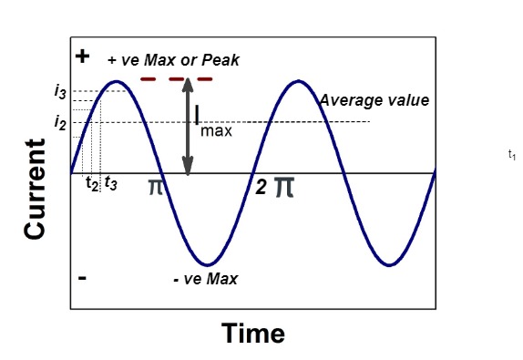
Fig. Sinusoidal waveform

The arithmetic means of all the value over complete one cycle is called as average value

=

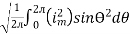
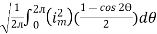
For the derivation we are considering only hall cycle.

Thus varies from 0 to ᴫ

i = Im   Sin

Solving

We get

Similarly, Vavg=

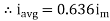
The average value of sinusoid ally varying alternating current is 0.636 times maximum value of alternating current.

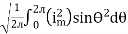
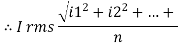
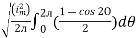
RMS value: Root mean square value

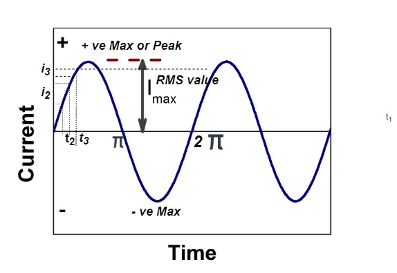
Fig. Sinusoidal waveform

The RMS value of AC current is equal to the steady state DC current that required to produce the same amount of heat produced by ac current provided that resistance and time for which these currents flows are identical.

I rms =  

Direction for RMS value:

Instantaneous current equation is given by

i = Im Sin

but

I rms =  

=  

=

=

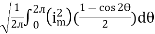
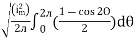
Solving

=

=

Similar we can derive

V rms= or 0.707 Vm

the RMS value of sinusoidally alternating current is 0.707 times the maximum value of alternating current.

3.2 Phasor diagrams

The alternating quantities (voltages and currents) in practice are represented by straight lines having definite direction and length. Such lines are called the phasors and the diagrams in which phasors represent currents, voltages and their phase difference are known as phasor diagrams.

Though phasor diagrams can be drawn to represent either maximum or effective values of voltages and currents but since effective values are of much more importance, phasor diagrams are mostly drawn to represent effective values.

In order to achieve consistent and accurate results it is essential to follow certain conventions.

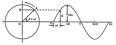
Fig. Phasor Diagram

The above figure shows that OA is the maximum ac quantity present. The OA represents emf on vertical axis. This phasor of OA in ACW direction represents sinusoidal voltage or current. Its angular velocity is one revolution complete in same time as by the alternating voltage or current.

The ACW is taken positive for phasor. In series circuit current phasor is taken as reference as the current is same. In parallel circuit voltage is taken as reference as it is same throughout.

3.3 Impedances and admittances

Impedances

The ac circuit is to always pure R pure L and pure C it well attains the combination of these elements. “The combination of R1 XL and XC is defined and called as impedance represented as 

Z = R +i X

Ø = 0

  only magnitude

R = Resistance, i = denoted complex variable, X =Reactance XL or Xc

Polar Form

Z   = L I

Where =

Measured in ohm

Admittances

The reciprocal of impedance is admittance. Its unit is mho (siemens)

Y= =

V=IZ

I=VY

Y= =

Y= G+iB

G=

B=

3.4 AC circuit analysis

Ac circuit containing pure resisting

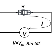
Consider Circuit Consisting pure resistance connected across ac voltage source

V = Vm Sin ωt      ①

According to ohm’s law i = = 

But Im =

②

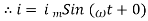
Phase’s diagram

From ① and ②phase or represents RMD value.

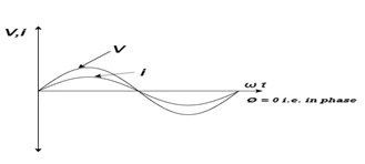
Fig. Phasor Diagram

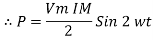
Power      P = V. i

Equation P = Vm sin ω t       Im sin ω t

P = Vm Im Sin2 ω t

P =   -

Constant fluctuating power if we integrate it becomes zero

Average power

Pavg =

Pavg =

Pavg = Vrms Irms

Power form [Resultant]

Fig. Resultant Power

Ac circuit containing pure Inductors

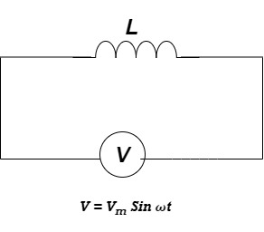
Fig. Inductive circuit

Consider pure Inductor (L) is connected across alternating voltage. Source

V = Vm Sin ωt

When an alternating current flow through inductance it set ups alternating magnetic flux around the inductor.

This changing the flux links the coil and self-induced emf is produced

According to faradays Law of E M I

e =

at all instant applied voltage V is equal and opposite to self-induced emf [ lenz’s law]

V = -e

=

But V = Vm Sin ωt

dt

Taking integrating on both sides

dt

dt

(-cos )

but sin (– ) = sin (+ )

sin ( - /2)

And Im=

/2)

/2

= -ve

= lagging

= I lag v by 900

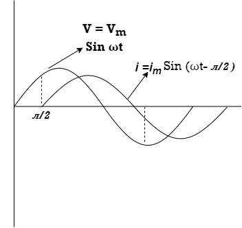
Fig. Voltage and Current waveform

Phasor:

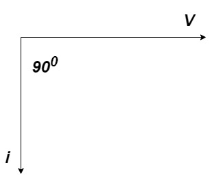
Fig. Phasor for L circuit

Power P = Ѵ. I

= Vm sin wt    Im sin (wt /2)

= Vm Im Sin wt Sin (wt – /s)

①

And

Sin (wt - /s) = - cos wt         ②

Sin (wt – ) = - cos

sin 2 wt    from ① and ②

The average value of sin curve over a complete cycle is always zero

Pavg = 0

Ac circuit containing pure capacitors:

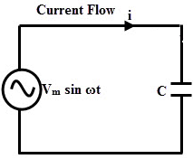
Fig. Pure Capacitive Circuit

Consider pure capacitor C is connected across alternating voltage source

Ѵ = Ѵm Sin wt

Current is passing through capacitor the instantaneous charge ɡ produced on the plate of capacitor

ɡ = C Ѵ

ɡ = c Vm sin wt

the current is rate of flow of charge

i=  (cvm sin wt)

i = c Vm w cos wt

then rearranging the above eqn.

i =     cos wt

= sin (wt + X/2)

i = sin (wt + X/2)

but

X/2)

= leading

= I leads V by 900

Waveform:

Fig. V_I waveform

Phase

Fig. Phasor for C circuit

Power   P= Ѵ. i

= [Vm sinwt] [ Im sin (wt + X/2)]

= Vm Im Sin wt Sin (wt + X/2)]

(cos wt)

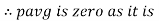to charging power waveform [resultant].

Fig. Power Waveform

3.5 Effective or RMS values

RMS value: Root mean square value

The RMS value of AC current is equal to the steady state DC current that required to produce the same amount of heat produced by ac current provided that resistance and time for which these currents flows are identical.

I rms =  

Direction for RMS value:

Instantaneous current equation is given by

i = Im Sin

but

I rms =  

=  

=

=

Solving

=

=

Similar we can derive

V rms= or 0.707 Vm

the RMS value of sinusoidally alternating current is 0.707 times the maximum value of alternating current.

3.6 Average power and complex power

Real Power: [P]

  It is nothing but the actual power being used in a circuit.

P= = I2R                          Watts

Reactive Power: [Q]

It is the function of reactance in the circuit X. Mainly reactive loads are inductor and capacitors. These elements dissipate zero power. These element shows that they dissipate power. This is called as reactive power.

Q= = I2X                          VAR (volt-Ampere-Reactive)

Apparent Power: [S]

It is the product of a circuit voltage and current without reference to phase angle. It is the combination of both reactive and real power.

S= = I2Z                            VA (volt-Ampere)

Power factor (P.F.)

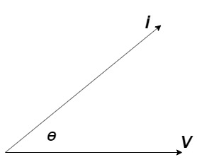
Fig. Power Factor

It is the cosine of angle between voltage and current

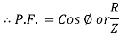
If Ɵ is –ve or lagging (I lags V) then lagging P.F.

If Ɵ is +ve or leading (I leads V) then leading P.F.

If Ɵ is 0 or in phase (I and V in phase) then unity P.F.

Examples

Que) A coil takes a current of 6A when connected to 24V dc supply. To obtain the same current with 50HZ ac, the voltage required was 30V. Calculate inductance and p.f of coil?

Sol: The coil will offer only resistance to dc voltage and impedance to ac voltage

R =24/6 = 4ohm

Z= 30/6 = 5ohm

XL =

    = 3ohm

cosφ = = 4/5 = 0.8 lagging

Que) The potential difference measured across a coil is 4.5V, when it carries a dc current of 8A. The same coil when carries ac current of 8A at 25Hz, the potential difference is 24V. Find current and power when supplied by 50V,50Hz supply?

Sol: R=V/I= 4.5/8 = 0.56ohm

At 25Hz Z= V/I=24/8 =3ohm

XL =

= 2.93ohm

XL = 2fL = 2x 25x L = 2.93

L=0.0187ohm

At 50Hz

XL = 2x3 =6ohm

Z = = 5.97ohm

I= 50/5.97 = 8.37A

Power = I2R = 39.28W

Que) A coil having inductance of 50mH an resistance 10ohmis connected in series

with a 25F capacitor across a 200V ac supply. Calculate resonant frequency and current flowing at resonance?

Sol: f0= = 142.3Hz

I0 = V/R = 200/10 = 20A

Que) A 15mH inductor is in series with a parallel combination of 80ohm resistor and 20F capacitor. If the angular frequency of the applied voltage is 1000rad/s find admittance?

Sol: XL = 2fL = 1000x15x10-3 = 15ohm

 XL = 1/C = 50ohm

Impedance of parallel combination Z = 80||-j50 = 22.5-j36

Total impedance = j15+22.5-j36 = 22.5-j21

Admittance Y= 1/Z = 0.023-j0.022 siemens

Que) A circuit connected to a 100V, 50 Hz supply takes 0.8A at a p.f of 0.3 lagging. Calculate the resistance and inductance of the circuit when connected in series and parallel?

Sol: For series Z =100/0.8 = 125ohm

cosφ =

R = 0.3 x 125 = 37.5ohm

XL = = 119.2ohm

 XL = 2fL = 2x 50x L

119.2 = 2x 50x L

L= 0.38H

For parallel:

Active component of current = 0.8 cosφ = 0.3x0.3 = 0.24A

R = 100/0.24 =416.7ohm

Quadrature component of current = 0.8 sinφ = 0.763

XL= 100/0.763 = 131.06ohm

L= 100/0.763x2x50 = 0.417H

Que) For a series RLC circuit having R=10ohms, L= 0.15H, C=100F. They are connected across 100v 50Hz supply. Calculate total impedance?

Sol: Impedance Z=

                             Z= 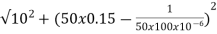= 18.27ohm

Que) For a series RLC circuit having R=12ohms, L= 0.2H, C=60F. They are connected across 100v 50Hz supply. Calculate circuit current?

Sol: I=

Z=

Z= 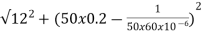= 13.89ohm

I = 100/13.89 =7.2A

Que) For a series RLC circuit having R=10ohms, L= 0.15H, C=100F. They are connected across 100v 50Hz supply. Calculate power factor?

Sol: cosφ =

Impedance Z=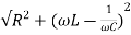

                             Z= = 18.27ohm

cosφ = =

φ = 56.81o lagging

3.7 Three-phase circuits

In three phase the windings are separated by 1200 each. The voltage produced in those windings are 1200 apart from each other. Below shown is one coil RR’ and two more coils YY’ and BB’ each having phase shift of 1200.

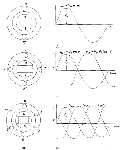
Fig. Three phase circuit waveform

The instantaneous value of voltages is given as

VRR’ = Vmsinωt

VYY’ = Vmsin(ωt-120)

VBB’ = Vmsin(ωt-240)

The three phase voltages are of same magnitude and frequency.

Phase sequence

The change in voltage is in order VRR’- VYY’- VBB’. So, the three-phase are changed in that order and are called as phase change.

VRR’ = Vmsinωt

VYY’ = Vmsin(ωt-120)

VBB’ = Vmsin(ωt-240)

3.8 Mutual coupled circuits and Dot Convention in coupled circuits

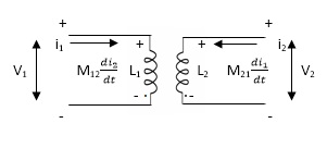
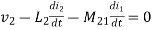
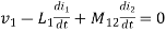
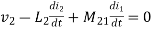
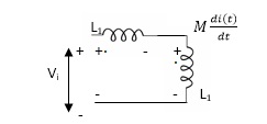
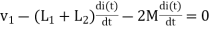
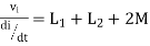
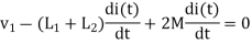
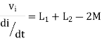
MUTUAL INDUCTANCE: -

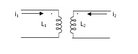
Fig. Mutual Inductance

M12= mutual inductance on 1 due to 2

M21= mutual inductance on 2 due to 1

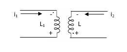
Fig. Current entering both dots

voltage on 2 due to 1 =

voltage on 1 due to 2 =

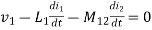
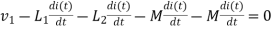
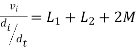
1. When current is entering or leaving from both dots.

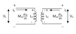
Fig. Current entering both dots

       ⎼⎼⎼⎼⎼⎼ 1

        ⎼⎼⎼⎼⎼⎼2

       ⎼⎼⎼⎼⎼⎼⎼1

              ⎼⎼⎼⎼⎼⎼⎼2

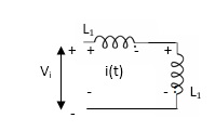
2. When current is entering from one dot and leaving the other

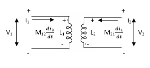
Fig. Current entering one dot and leaving other

        ⎼⎼⎼⎼⎼⎼⎼⎼1

        ⎼⎼⎼⎼⎼⎼⎼⎼2

3. When current is entering in both dots

Find =?

Fig. Current enters both dots

If M12= M21= M

4. When current leaves both dots

Find

Fig. Current Leaving both dots

5. When current enters from L1 and leaves L2

Find

Fig. current enters from L1 and leaves L2

6. When current leaves L2and enters L1

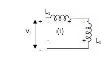
Fig. current leaves L2and enters L1

Key takeaway

The current entering the dot is taken as positive.

Example 1. Find

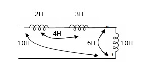
= 2H + 3H +10H - 2(10H) + 2(4H) + 2(6H)

= 15H + - 20H + 20H

= 0

Example 2. Find

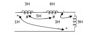
5H + 6H + 9H - 2(1H) -2(5H) -2(3H)

= 2H

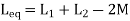
PARALLEL COMBINATION: -

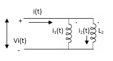
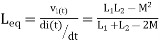
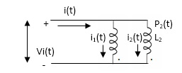
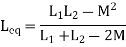
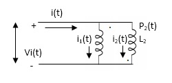
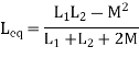
Fig. Parallel Combination

3.9 Ideal Transformer

An ideal transformer has no losses i.e., its winding has no magnetic leakage and no ohmic resistance. Hence, an ideal transformer has only two purely inductive coils wound on a loss-free core.

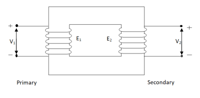
Fig. Ideal   Transformer

For above transformer when secondary is open and primary is having input sinusoidal voltage V1. An alternating current flow due to difference in potential. As primary coil is purely inductive so, Iµ current is drawn through it. This current is very small and logs V1 by 900.

The current Iµ produces magnetic flux φ and hence are in same phase. The flux is linked with both the windings and hence, self-induced emf is produced E1 which is equal and opposite of V1. Similarly, E2 is induced in secondary which is mutually induced emf E2 is proportional to rate of change of flux and number of secondary windings.

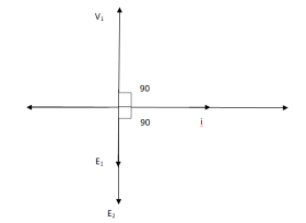
The phasor is shown below.

                                            Fig. Phasor for Ideal Transformer

Emf Equation of Transformer:

N1 = No of primary turns

N2 = No of secondary turns

Φm = max flux in cone (wb)

Φm = Bm x A

f = Frequency of input(ac) Hz

Average rate of change of flux

= Φm / ¼ 

= 4 ΦmF volts

Average emf per turn = 4F ΦmV

As Φ varies sinusoidally rms value of induced emf is given as

Form factor = r.m.s value / average value = 1.11

r.m.s value of emf/turn = 1.11 x 4f Φm

= 4.44 f Φm volt

r.m.s value of induced emf in primary winding

= (induced emf/turn) x No of primary turns

E1 = 4.44 fN1 Φm

E1 = 4.44 fN1BmA

r.m.s emf induced in secondary

E2 = 4.44 fN2 Φm

E2 = 4.44 fN2BmA

E1/E2 = N1/N2 = K

K – voltage transformation

(i). If N2 > N1 i.e., K > 1  STEP UP TRASFORMER

(II). If N1 > N2 i.e., K<1  STEP DOWN TRASFORMER

FOR Ideal Transformer

V1 I1 = V2 I2 = 1/K

Hence, current is inversely proportional to the voltage transformation ratio.

Key takeaway

r.m.s value of induced emf in primary winding E1 = 4.44 fN1 Φm

r.m.s emf induced in secondary E2 = 4.44 fN2 Φm

(i). If N2 > N1 i.e., K > 1  STEP UP TRASFORMER

(II). If N1 > N2 i.e., K<1  STEP DOWN TRASFORMER

FOR Ideal Transformer

V1 I1 = V2 I2 = 1/K

Q1>. A 25 KVA transformer has 500 turns on primary and 50 on secondary. The primary is connected to 2000V, 50 Hz supply. Find full load primary and secondary currents, the secondary emf and max flux in core. Neglect leakage drop and no load primary current.

Sol K = N2/N1 = 50/500 = 1/10

I1 = 25,000/2000 = 12.5 A

I2 = I1/K = 10 x 12.5 A = 125 A

Emf/turn on primary side = 2000/500 = 4 V

E2 = KE1

E2 = 4 x 50 = 200 v

E1 = 4.44fN1 Φm

2000 = 4.44 x 50 x 500 x Φm

Φm = 18.02 m Wb

References:

Education, 2013.

4.     C. K. Alexander and M. N. O. Sadiku, “Electric Circuits”, McGraw Hill Education, 2004.

5.      K. V. V. Murthy and M. S. Kamath, “Basic Circuit Analysis”, Jaico Publishers, 1999.