Unit - 1
Discrete Time System
Discrete time signal:
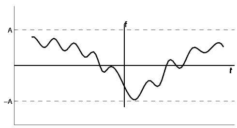
If a discrete variable x(t) is defined at discrete time then x(t) is a discrete time signal. A discrete time signal is often identified as a sequence of number denoted by x(n), where ‘n’ is an integer.
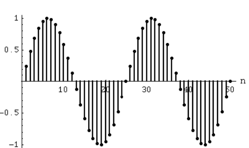
Fig:1 Discrete time signal
Even and Odd Signals
The even signals are symmetrical about Y-axis. They lie in first and second quadrants.
x[-n]=x[n]
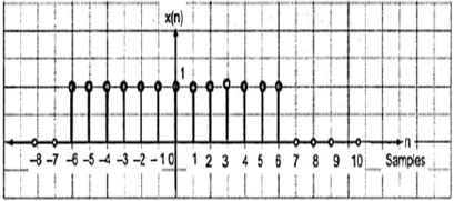
Fig:2 Even signal
The odd signals are symmetrical about origin. They lie in first and third quadrants.
x[-n]= -x[n]
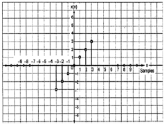
Fig:3 Odd signal
A signal having even and odd parts is mixed signal.
Periodic and Non-periodic signals:
A signal which repeats itself after a particular period of time is called as Periodic signal. The condition for any signal to be periodic is
x(n+N) = x(n)
considering a cosine signal −
x(n)=A cos(2πf0n+θ) x(n)= A cos(2πf0n+θ)
x (n +N) = A cos (2πf0(n +N) +θ)
=A cos(2πf0n+2πf0N+θ) x (n+ N)
=A cos (2πf0(n +N) +θ) =A cos(2πf0n+2πf0N+θ)
=A cos(2πf0n+2πf0N+θ) = A cos(2πf0n+2πf0N+θ)
For the signal to become periodic, following condition should be satisfied;
X (n+ N) = x(n) x (n +N) = x(n)
A cos(2πf0n+2πf0N+θ) =A cos(2πf0n+θ)
A cos(2πf0n+2πf0N+θ) = A cos (2πf0n+ θ)
As, 2πf0N is an integral multiple of 2π
2πf0N=2πK
N=Kf0
Frequencies of discrete sinusoidal signals are separated by integral multiple of 2π.
Energy and Power Signals
Energy Signal
Energy of a discrete time signal is denoted as E. It can be written as
E = 
If each individual values of x(n)x(n) are squared and added, we get the energy signal. Here x(n) is the energy signal and its energy is finite over time i.e 0<E<∞
Power Signal
Average power of a discrete signal is represented as P. This can be written as
P = 

Key takeaway
E = 
P = 

1) Linear and Non-Linear system:
A system is said to be linear when it obeys law of superposition.
If we have two inputs x1(n) and x2(n), and output y(n). The operator ‘H’ is called linear operator if it satisfies the following condition.

Fig 4 Input first pass through adder
In the above figure first the two inputs pass through an adder than through the operator. So, the equation after adder will be ax1(n)+bx2(n). Now final output equation after passing through operator is
Y(n)=H[ax1(n)+bx2(n)]=Hax1(n)+H bx2(n)
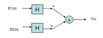
Fig 5 Input first pass through operator
Now, in above figure the two inputs first pass through the operator and then through the summer. The equation at output is
Y(n)= Hax1(n)+H bx2(n)
The two output equations in both the systems are same. Hence, the system operator H is linear.
Non-Linear system: If the system does not obey law of superposition, it is said to be non-linear.
2) Time variant and Time Invariant system: A time delay or advance in the input signal produces the corresponding change in the output. Then the system is said to be time invariant.


Fig:6 Time-Invariant system
If the delay or advance in the system does not produce corresponding change in the output then it’s called as Time variant System.
3) Causal and Anti-Causal system: A system is said to be causal if it’s output at any point of time depends only on the input x(t) for time ‘t’, where t<t0, where t0 is the present time. If not so then it is called as anti-causal system.
Only causal signals are realisable signals.
4) Memory and Memoryless System: A system is said to be memoryless if at any point of time the output depends only on present input but not on its past inputs.
If the system output at instance of time depends on the past inputs then it is called as memory system.
5) Invertible and Non-Invertible system: The system is said to be invertible if the input of the system can be recovered from the system output.
Key takeaway
Only causal signals are realisable signals
Que) For the system with y(t)=x(-t), find whether the system is linear or not?
Sol: To comment on linearity of system it should follow law of superposition. So, From model given below
Y(t)=ax1(-t)+bx2(-t)
Now from second model
Y(t)= ax1(-t)+bx2(-t)
Since, output from both the model is same so system is linear.
Que) For y(t)=cos[x(t)], comment whether it is time invariant or not?
Sol: From model 1


Y(t)=cos[x(t-t0)]
From model 2


Y(t)=cos[x(t-t0)]
Since, time delay or advance in the input signal produces the corresponding change in the output. Hence, it is time invariant.
Que) For y(t)=x(t2), is the system causal or anti causal?
Sol: y(t)= x(t2)
If the output for any time depends on the future than its not causal. So, Let t=1
Y(1)=x(1)
t=2
y(2)=x(4)
Since, it depends on future values, so it is anti-causal.
Que) For y(t)=x(t)+2. Comment whether system has memory or memoryless?
Sol: For t=1
Y(1)=x(1)+2
For t=2
Y(2)=x(2)+2
So, for any value of t the output depends only on present input. Hence, it is memoryless.
BIBO stability stands for bounded input, bounded output stability. BIBO stability is the system property that any bounded input yields a bounded output. This is to say that as long as we input a signal with absolute value less than some constant, we are guaranteed to have an output with absolute value less than some other constant.
In order to understand this concept, we must first look more closely into exactly what we mean by bounded. A bounded signal is any signal such that there exists a value such that the absolute value of the signal is never greater than some value. Since this value is arbitrary, what we mean is that at no point can the signal tend to infinity, including the end behaviour.
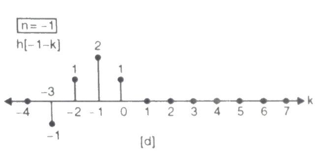
Fig 7 Discrete time BIBO Stable System
Now that we have identified what it means for a signal to be bounded, we must turn our attention to the condition a system must possess in order to guarantee that if any bounded signal is passed through the system, a bounded signal will arise on the output. It turns out that a continuous-time LTI system with impulse response h[n] is BIBO stable if and only if it is absolutely summable. That is
Discrete-Time Condition for BIBO Stability

In the z-domain is about as easy to demonstrate as it is for continuous-time signals in the Laplace domain. However, instead of the region of convergence needing to contain the jω-axis, the ROC must contain the unit circle. Consequently, for stable causal systems, all poles must be within the unit circle.
Key takeaway
Bounded input bounded output stability, also known as BIBO stability, is an important and generally desirable system characteristic. A system is BIBO stable if every bounded input signal result in a bounded output signal, where boundedness is the property that the absolute value of a signal does not exceed some finite constant. In terms of time domain features, a discrete time system is BIBO stable if and only if its impulse response is absolutely summable. Equivalently, in terms of z-domain features, a continuous time system is BIBO stable if and only if the region of convergence of the transfer function includes the unit circle.
Considering an LTI system with input as impulse signal. As we know that impulse response of any system gives complete describes the behaviour of any LTI system. Basically, we decompose the input signal first. The apply input as impulse and obtain the corresponding output. Obtained output is then graphically analysed.
Let input signal be x[n]
x[n] = 
The output obtained when we apply input as unit sample sequence for n=k
y[n,k] = h[n,k] = H[ [n-k]]
where n= time index
k = location of input impulse parameter
The x[n] because of input weighted sum of output will be
y[n] = H[x[n]]
= H [  ]
]
But y[n,k] = h[n,k] = H[ [n-k]]
Hence, the output will now be
y[n] = [  ]
]
=  ] (Due to superposition theorem)
Now, by time invariance property we can write
h[n]= H [
For delayed sequence we have
h[n-k] =H [ ]
]
Hence, the output equation can now be written as
y[n] = [  ]
]
The above equation is called as convolution sum.
y[n]= x[n] * h[n]
Key takeaway
y[n] = [  ]
]
The above equation is called as convolution sum
Example

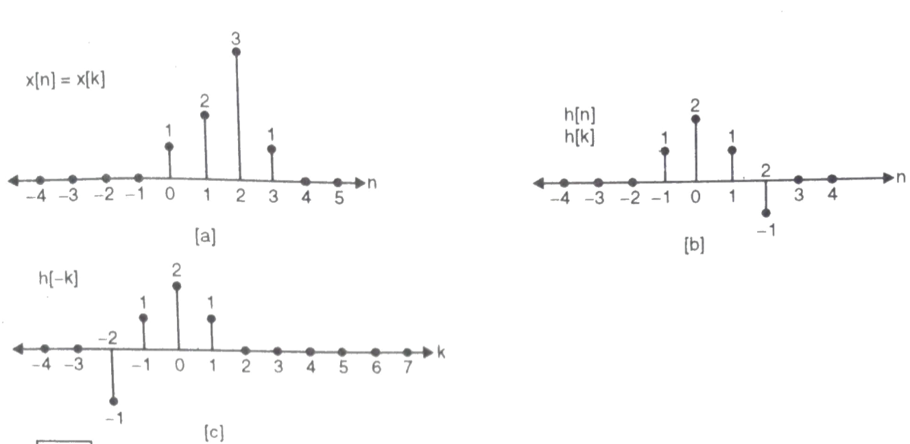
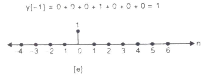
 Que) For sequence h[n]={ 1, 2 , 1, -1} determine the response of system with input signal x[n] = {1, 2 ,3 ,1}
Sol:
a) Finding x[k] and h[k] i.e n=k.
b) Folding h[k] we get h[-k].
c) Then shifting the above signal[-k] we get h[1-k]
d) Multiplying above signal h[1-k] with x[n].
e) Again, incrementing h[1-k] by 1 we get h[2-k] multiplying with x[n].
f) Continuing this process till we get 0 for output y. In this case for n=5.
The graphical representation is shown below.
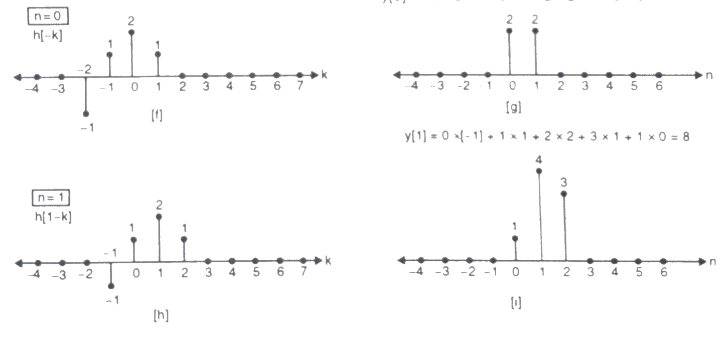
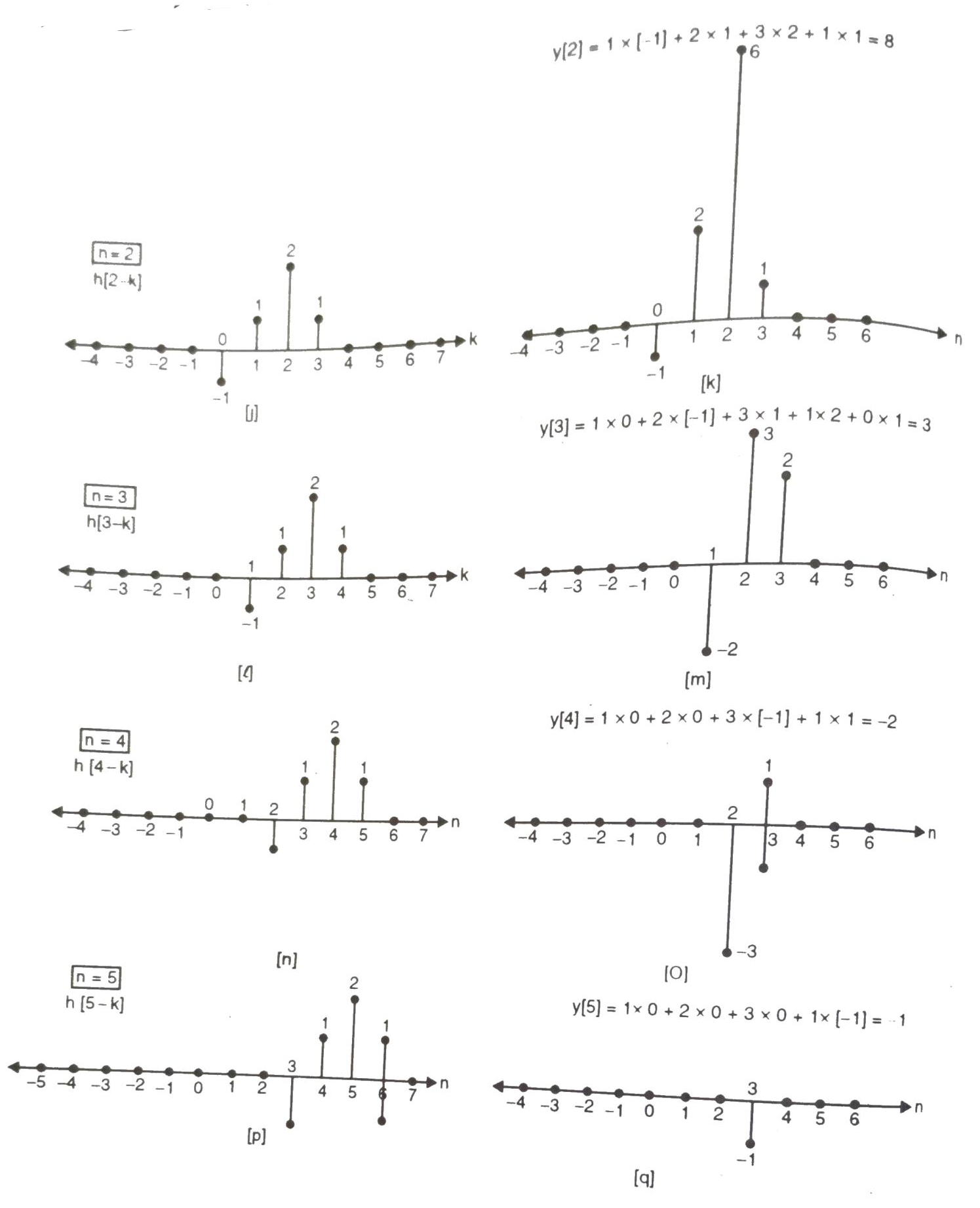

Convolution by tabulation method
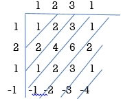
In this method we form a table type structure and find the convolution of x[n] and h[n]. We will understand this by solving an example.

 Que) For h[n] = {1, 2, 1, -1}, x[n] = {1, 2, 3, 1}. Find x[n]*h[n]?
Sol:
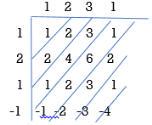
y[-1] = 1
y[0]= 2+2 = 4
y[1] = 1+4+3 = 8
y[2]= -1+2+6+1 = 8
y[3]= -2+3+2 = 3
y[4]= -3+1 = -2
y[5]= -1
 y[n]= {1, 4, 8, 8, -2, -1}
The above sequence is the required convolution of x[n] and h[n].
A recursive system is a system in which current output depends on previous output(s) and input(s) but in non-recursive system current output does not depend on previous output(s).
The system with memory is not necessarily a recursive system. For example: in FIR systems for input x[n] and output y[n] if we have
y[n] = 0.5(x[n]+x[n-1]) then the current output does not depend on previous output but depends on current input and previous input. But for IIR case like an accumulator
y[n] = y[n-1] + x[n], current output is depended on previous output as well as on current input (generally current and previous inputs). So, accumulator is a recursive system.
The LTI system can be represented by its impulse response with x(t) as its input signal and y(t) as its output.

Fig 8 LTI System
Let input signal be x[n]
x[n] = 
The output obtained when we apply input as unit sample sequence for n=k
y[n,k] = h[n,k] = H[ [n-k]]
y[n] = H[x[n]]
= H [  ]
]
But y[n,k] = h[n,k] = H[ [n-k]]
Hence, the output will now be
y[n] = [  ]
]
=  ]
]
Correlation means to correlate two signals or processes. In correlation we just reverse one of the sequences. There are two types in which we can correlate signals as mentioned below.
Mathematically correlation can be defined as
rxy(l) = 

rxy(l) = 

a) Cross-correlation of x(n) and y(n) is a sequence, rxy(l)
rxy(l) =  l= 0, ±1, ±2,….
rxy(l) =  l= 0, ±1, ±2,….
After Reversing x and y we get, ryx(l)
ryx(l) =  l= 0, ±1, ±2,….
ryx(l) =  l= 0, ±1, ±2,….
Que) Determine the cross-correlation sequence rxy(l) of sequence
 x[n] = {…… 0, 0, 0, -3, -2 ,1, 4, 8, -3, 0 ,0 ,0 ….}
 y[n] = {…… 0, 0, 0, 1, 1, -1, 2, -2, 0 ,0 ,0 ….}
Sol: The cross-correlation is given as
rxy(l) =  l= 0, ±1, ±2,….
For l=0
rxy(l) = 
 M[n] = {…… 0, 0, 0, -3, -2 ,-1, -4, 16, 6, 0 ,0 ,0 ….}
For l=1
rxy(l) = 
 x[n] = {-3, -2 ,1, 4, 8, -3}
 y[n]= {0, 1, 1, -1, 2, -2, 0}
 y[n-1] = {0, 1, 1, -1, 2, -2}
rxy(l) = rxy(+1) =  = -11
= -11
For l= 2
 x[n] = {-3, -2 ,1, 4, 8, -3}
 y[n-2] = { 0,0, 1, 1, -1, 2, -2, 0}
rxy(l) = rxy(+2) =  = 16
= 16
For l= 3
 x[n] = {-3, -2 ,1, 4, 8, -3,0,0,0…}
 y[n-3] = {0, 0,0, 1, 1, -1, 2, -2, 0}
rxy(l) = rxy(+3) =  = 9
= 9
For l = 4
x[n] = {-3, -2 ,1, 4, 8, -3,0,0,0…}

 y[n-4] = {0,0, 0,0, 1, 1, -1, 2, -2, 0}
rxy(l) = rxy(+4) =  = 5
= 5
For l=5
 x[n] = {-3, -2 ,1, 4, 8, -3,0,0,0…}
 y[n-5] = {0,0,0, 0,0, 1, 1, -1, 2, -2, 0}
rxy(l) = rxy(+5) =  = -3
= -3
For l>6
rxy(l) = 0
Similarly finding for l= -1, -2,……
rxy(-l) = -14
rxy(-2) = -7
rxy(-3) = -3
rxy(-4) = -2
rxy(-5) = 6
rxy(-6) = 0
rxy(l) = {6, -2, -3, -7, -14, 14, -11, 16, 9, 5, -3}
b) Auto Correlation: Here we correlate the signal with itself.
rxx(l) =  l= 0, ±1, ±2,….
rxx(l) =  l= 0, ±1, ±2,….
 Que) Auto-correlate x[n] = {1,2,1,1}
Sol: rxx(l) = 
For l=0
rxx(0) = 
=1x1+2x2+1x1+1x1=7
For l=1
rxx(1) = 
x[n-1] = {0,1,2,1,1}
rxx(1) = 5
For l=2
rxx(2) = x[n-2] = {0,0,1,2,1,1}
rxx(2) = 5
For l=3
rxx(3) = x[n-3] = {0,0,0,1,2,1,1}
rxx(3) = 1
rxx(-1) = 
For l=-1
x[n+1] = {1,2,1,1,0}
rxx(-1) = 5
For l= -2
rxx(-2) = x[n+2] = {1,2,1,1,0,0}
rxx(-2) = 2
For l= -3
rxx(-3) = x[n+3] = {1,2,1,1,0,0,0}
rxx(-3) = 1
 rxx(l) = {1,3,5,7,5,3,1}
Reference