Unit - 3
Discrete Fourier Transform
Frequency domain sampling
Sampling in frequency domain is usually used in DFT (Discrete Fourier transform), where continuous signal of spectrum in sampled to get discrete values of spectrum, which results in periodicity in time domain. This helps to process any continuous spectrum signal of non periodic in nature to discretize and digitize for further processing.
The following figure indicates a continuous-time signal x (t) and a sampled signal xs (t). When x (t) is multiplied by a periodic impulse train, the sampled signal xs (t) is obtained.
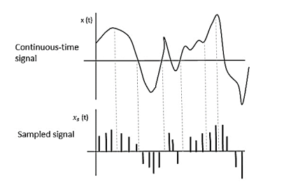
Fig 1 Sampled Signal
Sampling Rate
To discretize the signals, the gap between the samples should be fixed. That gap can be termed as a sampling period Ts.
Sampling Frequency=1/Ts=fs
Where,
- Ts is the sampling time
- Fs is the sampling frequency or the sampling rate
Sampling frequency is the reciprocal of the sampling period. This sampling frequency, can be simply called as Sampling rate. The sampling rate denotes the number of samples taken per second, or for a finite set of values.
Nyquist Rate
Suppose that a signal is band-limited with no frequency components higher than W Hertz. That means, W is the highest frequency. For such a signal, for effective reproduction of the original signal, the sampling rate should be twice the highest frequency.
Which means,
fS=2W
Where,
- fS is the sampling rate
- W is the highest frequency
This rate of sampling is called as Nyquist rate.
Sampling theorem in time domain
The sampling theorem, which is also called as Nyquist theorem, delivers the theory of sufficient sample rate in terms of bandwidth for the class of functions that are bandlimited.
The sampling theorem states that, “a signal can be exactly reproduced if it is sampled at the rate fs which is greater than twice the maximum frequency W.”
Let us consider a band-limited signal, i.e., a signal whose value is non-zero between some –W and W Hertz.
Such a signal is represented as x(f)=0 for ∣f∣>W
For the continuous-time signal x (t), the band-limited signal in frequency domain, can be represented as shown in the following figure.
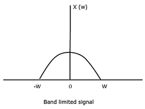
Fig 2 Band Limited Signal
If the signal x(t) is sampled above the Nyquist rate, the original signal can be recovered, and if it is sampled below the Nyquist rate, the signal cannot be recovered.
The following figure explains a signal, if sampled at a higher rate than 2w in the frequency domain.
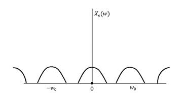
Fig 3 fs>2W
The above figure shows the Fourier transform of a signal xs (t).
If fs<2W
The resultant pattern will look like the following figure.
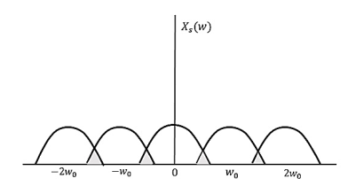
Fig 4 fs<2W
Here, the over-lapping of information is done, which leads to mixing up and loss of information. This unwanted phenomenon of over-lapping is called as Aliasing.
Aliasing
Aliasing can be referred to as “the phenomenon of a high-frequency component in the spectrum of a signal, taking on the identity of a low-frequency component in the spectrum of its sampled version.”
Numerical:
- The continuous-time signal x(t) = cos(200πt) is used as the input for a CD converter with the sampling period 1/300 sec. Determine the resultant discrete-time signal x[n].
Solution:
We know,
X[n] =x(nT)
= cos(200πnT)
= cos(2πn/3) , where n= -1,0,1,2……
The frequency in x(t) is 200π rad/s while that of x[n] is 2π/3.
2. Determine the Nyquist frequency and Nyquist rate for the continuous-time signal x(t) which has the form of:
X(t) = 1+ sin(2000πt) + cos (4000πt)
Solution:
The frequencies are 0, 2000π and 4000π.
The Nyquist frequency is 4000π rad/s and the Nyquist rate is 8000π rad/s.
3) Consider an analog signal.

Solution.
The frequency in the analog signal

The largest frequency is

The Nyquist rate is

4) The analog signal

- What is the Nyquist rate for this signal?
- Using a sampling rate
 . What is discrete time signal obtained after sampling?
 - What is analog signal
 we can reconstruct from the samples if we use ideal interpolation?
Solution.
- The frequency of the analog signal are


2. For 


For  ,the folding frequency is
Hence  is not affected by aliasing
 Is changed by the aliasing effect
 Is changed by the aliasing effect
So those normalizing frequencies are

The analog signal that we can recover is

Which is different than the original signal 
5) For 
- Find the minimum sampling rate required to avoid aliasing.
- If
 , what is the discrete time signal after sampling?
 - If
 , what is the discrete time signal after sampling?
 - What is the frequency F of a sinusoidal that yields sampling identical to obtained in part c?
Solution.
a. 
The minimum sampling rate is

And the discrete time signal is

b. If  , the discrete time signal is

c. If Fs=75Hz , the discrete time signal is

d. For the sampling rate 
 in part in (c). Hence

So, the analog sinusoidal signal is


6) Suppose a continuous-time signal x(t) = cos (Ø0t) is sampled at a sampling frequency of 1000Hz to produce x[n]: x[n] = cos(πn/4). Determine 2 possible positive values of Ø0, say, Ø1 and Ø2. Discuss if cos(Ø1t) or cos(Ø2t) will be obtained when passing through the DC converter.
Solution:
Taking T= 1/1000s
Cos(πn/4) =x[n] = x(nT) = cos (Ø0n/1000)
Ø1 is easily computed as 
Ø1 = 250π
Ø2 can be obtained by noting the periodicity of a sinusoid:
 Ø2n/1000)
Ø2 = 2250π
Reconstruction of Discrete-Time Signals
Reconstruction process
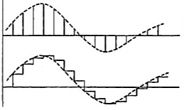
Fig 5 Reconstruction of signal
The sampled data signal is modified by the controller. The hold circuit than converts the signal to analog form. The simplest hold circuit is ZOH (zero order hold) in which the reconstructed signal acquires the same value as the last received sample for the entire sampling period.
The basic sampler is shown in above figure (a) and output in figure (b). The high frequency signal present in the reconstructed signal is filtered by the controller elements which are the low pass in frequency behaviour.
The first or higher order holds have no advantage over the ZOH. In the first order hold the last two signal samples are used to reconstruct the signal for the current sampling period.
Key takeaway
Aliasing can be referred to as “the phenomenon of a high-frequency component in the spectrum of a signal, taking on the identity of a low-frequency component in the spectrum of its sampled version.”
The discrete Fourier transform transforms a sequence of N complex numbers  into another sequence of complex numbers
 which is defined by


Example:
Let N =4 and

Here we demonstrate how to calculate the DFT of x using equation (1)


Using Linearity property, we can find the DFT easily. The formula for which is given as
X[K] =  =
= 
x[n] = 1/N  = 1/N
= 1/N 
WN = 
Suppose we have signal sequence x[n], then we will define vector xN of N point samples same way we will define vector N point for XN and WN.
xN =  XN =
XN = 
WN = 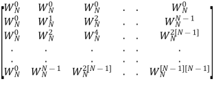
Thus, we can represent N point DFT in matrix form
XN = WN xN
Example
Compute 4-point DFT of given sequence {1,0,0,1}. Use matrix for DFT computation?
Sol: x[n] = {1,0,0,1}
N-1 = 3
N= 4
W4 =  =
= 
X4 = 
X4 = 
Relation to FT of an Aperiodic Sequence
A periodic sequence with FT X |ω| of aperiodic finite energy sequence x[n], sampled at N equally spaced frequencies.
ωk =2πk/N for 0≤k≤N-1
X[k]= X [ω] for ω = 2πk/N = 
Relation with Fourier coefficients of a Periodic Sequence
A periodic sequence x[n] with fundamental period N can be represented in Fourier series
x[n] = 
ck = 1/N 
DFT and the above equation when compared we get
X[k] = 
DFT sequence is given by X[k] = N Ck
x[n] = 1/N 
Thus, N point DFT provides exact line spectrum of a periodic sequence with fundamental period N.
Relation with Z-transform
Z-transform is given as
X[z] = 
z= 
X[z] = 
The above equation is same as X[k] except the limits of n. So, if x[n] has finite duration length N we can write
X[z]=  =
= 
It means that X[z] for z= is equal to X[k]
We can express X[z] as a function of DFT X[k] as
X[ω] = 

Key takeaway
DFT sequence is given by X[k] = N Ck
x[n] = 1/N 
Thus, N point DFT provides exact line spectrum of a periodic sequence with fundamental period N.
Linear Property
If x(t) -> X(w)
Y(t) -> Y(w) then
a x(t) + b y(t) -> a X(w) +b Y(w)
Time Shifting Property
If x(t)⟷F.TX(ω)
Then Time shifting property states that
x(t−t0)⟷F.T e−jω0t X(ω)
Frequency Shifting Property
If x(t)⟷X(ω)
Then frequency shifting property states that
Ejω0t.x(t)⟷X(ω−ω0)
Time Reversal Property
If x(t)⟷X(ω)
Then Time reversal property states that
x(−t)⟷X(−ω)
Differentiation Property
If x(t)⟷X(ω)
Then Differentiation property states that
Dx(t)dt ⟷jω.X(ω)
dnx(t)dtn⟷(jω)n.X(ω)
Integration Property
Integration property states that
∫x(t)dt⟷1jω X(ω)
Then
∭...∫x(t)dt⟷(jω)n X(ω)
Multiplication and Convolution Properties
If x(t)⟷X(ω)
y(t)⟷Y(ω)
Then multiplication property states that
x(t).y(t)⟷X(ω)∗Y(ω)
And convolution property states that
x(t)∗y(t)⟷1/2πX(ω).Y(ω)
Key takeaway
Property | Time Domain | Frequency domain |
1. Linearity |  |  |
2. Time-shifting |  |  |
3. Frequency-shifting (modulation) |  |  |
4. Time reversal |  |  |
5. Conjugation |  |  |
6. Time-convolution |  |  |
7. Frequency-convolution |  |  |
8. Parseval’s relation |  |  |
Numerical:
- Compute the N-point DFT of x(n)=3δ(n).


2. Compute the N-point DFT of x(n)=7(n−n0)
Solution − We know that,

Substituting the value of x(n),

Multiplication of Two DFTs
It is nothing but circular convolution of two sequence which is discussed below.
Circular Convolution
Let us take two finite duration sequences  ,having integer length as N. Their DI are
  reapectively which is shown below


Now we will try to find the DFT of another sequence  , which is given by

By taking the IDFT of the above we get

After solving the above equation finally we get

Methods of Circular Convolution
Generally, there are two methods, which are adopted to perform circular convolution and they are −
- Concentric circle method
- Matrix multiplication method
Concentric Circle Method
Let x1(n) and x2(n) be two given sequences. The steps followed for circular convolution of x1(n) and x2(n) are
- Take two concentric circles. Plot N samples of x1(n) on the circumference of the outer circle maintaining equal distance successive points maintaining equal distance successive points in anti-clockwise direction.
- For plotting x2(n), plot N samples of x2(n) in clockwise direction on the inner circle, starting sample placed at the same point as 0th sample of x1(n)
- Multiply corresponding samples on the two circles and add them to get output.
- Rotate the inner circle anti-clockwise with one sample at a time.
Matrix Multiplication Method
Matrix method represents the two-given sequence x1(n) and x2(n) in matrix form.
- One of the given sequences is repeated via circular shift of one sample at a time to form a N X N matrix.
- The other sequence is represented as column matrix.
- The multiplication of two matrices give the result of circular convolution.
Numerical:
Perform circular convolution of the two sequences, x1(n)= {2,1,2,-1} and x2(n)= {1,2,3,4}

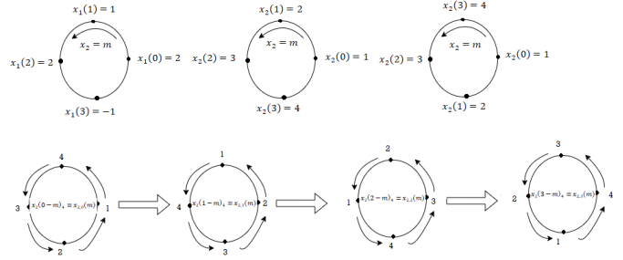
(2)

When n=0; 


The sum of samples of v0(m) gives x3(0)
x3(0)=2+4+6-2=10
When n=1; 


The sum of samples of v1(m) gives x2(1)
x3(1)=4 + 1 +8-3=10
(3) When n=2; 


The sum of samples of v2(m) gives x3(2)
⸫ x3(2)=6+2+2-4=6
(4) When n=3; 


The sum of samples of v3(m) gives x3(3)
⸫ x3(3)=8+ 3+ 4-1= 14
x3(n)={10,10,6,14}

 | -3 | -2 | -1 | 0 | 1 | 2 | 3 |
 |
|
|
| 2 | 1 | 2 | -1 |
 |
|
|
| 1 | 2 | 3 | 4 |
 | 4 | 3 | 2 | 1 | 4 | 3 | 2 |
 |
| 4 | 3 | 2 | 1 | 4 | 3 |
 |
|
| 4 | 3 | 2 | 1 | 4 |
 |
|
|
| 4 | 3 | 2 | 1 |


= x1(0) x x2,0(0) + x1(1) x2,0(1) + x1(2) x2,0(2) + x1(3) x2,0(3)
= 2 x 1 + 1 x 4 + 2 x 3 + (-1) x 2 = 2 +4 +6 -2 =10
Linear Convolution states that
y(n) = x(n) * h(n)


Example 1: h(n) = { 1 , 2 , 1, -1 } & x(n) = { 1, 2, 3, 1 } Find y(n).
METHOD 1: GRAPHICAL REPRESENTATION
Step 1) Find the value of n = nx+ nh = -1 (Starting Index of x(n)+ starting index of h(n))
Step 2) y(n)= { y(-1) , y(0) , y(1), y(2), ….} It goes up to length(xn)+ length(yn) -1. i.e n=-1


METHOD 2: MATHEMATICAL FORMULA
Use Convolution formula

k= 0 to 3 (start index to end index of x(n))
y(n) = x(0) h(n) + x(1) h(n-1) + x(2) h(n-2) + x(3) h(n-3)
METHOD 3: VECTOR FORM (TABULATION METHOD)
X(n)= {x1,x2,x3} & h(n) ={ h1,h2,h3}
|  |  |  |
 |  |  |  |
 |  |  |  |
 |  |  |  |
y(-1) = h1 x1
y(0) = h2 x1 + h1 x2
y(1) = h1 x3 + h2x2 + h3 x1 …………
METHOD 4: SIMPLE MULTIPLICATION FORM


The two methods used for filtering long sequences to short sequence are
Overlap-Save Method
The below figure shows this method. The steps involved are
- Size of data input block is N =L+M-1
- Size of DFT and IDFT are of length N
- Input data sequence is segmented into block of L points
- FIR filter response has duration M
- L>>M which means data sequence is longer than impulse response
- As length is L+M-1 data points in impulse response are increased in length by appending L-1 zeros
Impulse
Response
Sequence
L -1 zeros
h(n) | 0, ……….,0 |
h(0), …………, h (M -1)
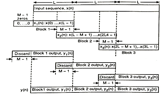
Fig 6 Overlap-Save Method
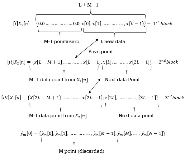
- Each data block consists of last M-1 data points of previous data block and L data points from data sequence follows it
- Multiplication of two N point DFT H[k] and Xm[k] for mth block of data
 [k] = H[k] Xm[k] for 0≤ k ≤ N-1
- N point DFT will be given as
 [n] = {ym(0), ym(1),…. ym(N-1)}
- Data record is of length N therefore, first M-1 points of ym[n] are corrupted by aliasing and must be discarded. The last L points are exactly same as result from linear convolution.
 =ym[n]
- To avoid loss of data due to aliasing last M-1 points of each data records are saved. The saved M-1 points become first M-1 data points of subsequent record. Initially M-1 points of first record are set to 0.
Example
The unit sample response sequence of a system h[n] = {3,2,1}. Use the overlap save method to determine its output sequence in response to the repeating input sequence {2,0,-2,0,2,1,0,-2,-1,0}. Take N=8.
Sol:
- h[n] = {3,2,1}, M=3, M-1 =2
- x[n] = {2,0,-2,0,2,1,0,-2,-1,0}
- If N = L+M-1= L+3-1
8=L+2
L=6
The length of block selected is 6.
 | -2 | -1 | 0 | 1 | 2 | 3 | 4 | 5 | 6 | 7 | 8 | 9 | 10 | 11 | … |
 |
|
| 2 | 0 | -2 | 0 | 2 | 1 | 0 | -2 | -1 | 0 | 2 | 0 | … |
 | (0 | 0) | 2 | 0 | -2 | 0 | 2 | 1 |
|
|
|
|
|
|
|
 |
|
|
|
|
|
| 2 | 1 | 0 | -2 | -1 | 0 | 2 | 0 |
|
 |
|
|
|
|
|
|
|
|
|
|
|
| 2 | 0 | … |
 Block 1
  Zeros added
 Block 2
 Block 3
- Pad L-1 zeros to h[n]. Therefore, sequence will be
h[n] = {3,2,1,0,0,0,0,0}
- Perform circular convolution of h[n] with x1[n] which is shown below
| Periodic extension of data block 1 | Data block 1 | ||||||||||||||
 | 0 | 2 | 0 | -2 | 0 | 2 | 1 | 0 | 0 | 2 | 0 | -2 | 0 | 2 | 1 | |
 | 0 | 0 | 0 | 0 | 0 | 1 | 2 | 3 |  |
|
|
|
|
|
| |
 |
|
|
|
|
|
|
| 4 | 1 | 6 | 4 | -4 | 4 | 4 | 7 | |
- Take block 2 and circular convolve with h[n] as shown below
| Periodic extension of data block 2 | Data block 2 | ||||||||||||||
 | 1 | 0 | -2 | -1 | 0 | 2 | 0 | 2 | 1 | 0 | -2 | -1 | 0 | 2 | 0 | |
 | 0 | 0 | 0 | 0 | 0 | 1 | 2 | 3 |  |
|
|
|
|
|
| |
 |
|
|
|
|
|
|
| 8 | 7 | 4 | -5 | -7 | 4 | 5 | 4 | |
- Add y1[n], y2[n] and so on but discard first two values from the answer and save last six values of each circular convolution as shown in figure below.
 | -2 | -1 | 0 | 1 | 2 | 3 | 4 | 5 | 6 | 7 | 8 | 9 | 10 | 11 | … |
 | 4 | 1 | 6 | 4 | -4 | -4 | 4 | 7 |
|
|
|
|
|
|
|
 |
|
|
|
|
|
| 8 | 7 | 4 | -5 | -7 | -4 | 5 | 4 |
|
 |
|
|
|
|
|
|
|
|
|
|
|
| X | X | … |
 |
|
| 6 | 4 | -4 | -4 | 4 | 7 | 4 | -5 | -7 | -4 | 5 | 4 | … |
Discard result
Fig 7 Final answer from overlap save method
Overlap-Add Method
- Size of input data block is L points.
- Size of DFT and IDFT is N = L+M-1
- To data block we append M-1 zeros as shown below.
Impulse
Response
Sequence
L -1 zeros
h(n) 0, ……….,0
h(0), …………, h (M -1)
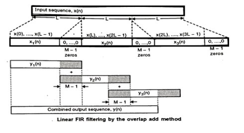
Fig 8 Linear FIR Filtering by overlap add method
 1st block
 2nd block
 3rd block
After multiplying impulse response of length of M with DFT of input sequence we get
Ym[k] = H[k] Xm[k]
Taking IDFT of Ym[k]. The output of IDFT is block of length M
N= L+M-1. The M-1 points from each output block must overlap and should be added to first M-1 points of succeeding block. The output sequence is given by
y1[n] = y1[0], y1[1],….y1[L-1],y1[L],y1[L+1]……..y1[L+M-1]
y2[n] = y2[0], y2[1],….y2[L-1],y2[L],y2[L+1]……..y2[L+M-1]
y[n] = y[0],y[1],……y[L-1],y[L],y[L+1]……..y[L+M-1]
Example
The unit sample sequence of a system is h[n] = {3,2,1}. Use overlap add method to determine its output sequence in response to the repeating input sequence {2,0,-2,0,2,1,0,0,-2,-1,0}. Take N=8.
Sol:
- h[n] = {3,2,1}, M=3, M-1 =2
- x[n] = {2,0,-2,0,2,1,0,-2,-1,0}
- If N = L+M-1= L+3-1
8=L+2
L=6
From input every time 6 elements are selected and two zeros (M-1) are padded after them as shown below.
 | 0 | 1 | 2 | 3 | 4 | 5 | 6 | 7 | 8 | 9 | 10 | 11 | 12 | 13 | … |
|
 | 2 | 0 | -2 | 0 | 2 | 1 | 0 | -2 | -1 | 0 | 2 | 0 | -2 | 0 | … |  |
 | 2 | 0 | -2 | 0 | 2 | 1 | 0 | 0 |
|
|
|
|
|
|
|  |
 |
|
|
|
|
|
| 0 | -2 | -1 | 0 | 2 | 0 | 0 | 0 |
|  |
 |
|
|
|
|
|
|
|
|
|
|
|
| -2 | 0 | … |  |
Fig 10 Breaking up long input sequence into blocks of data
- Pad L-1 zeros to h[n] sequence. Therefore, sequence will be
h[n] = {3,2,1,0,0,0,0,0}
- Perform circular convolution of h[n] with x1[n] which is shown below
| Periodic extension of data block 1 | Data block 1 |
| ||||||||||||||||
 | 0 | -2 | 0 | 2 | 1 | 0 | 0 | 2 | 0 | -2 | 0 | 2 | 1 | 0 | 0 |  | |||
 | 0 | 0 | 0 | 0 | 0 | 1 | 2 | 3 |  |
|
|
|
|
|
|   | |||
 |
|
|
|
|
|
|
| 6 | 4 | -4 | -4 | 4 | 7 | 4 | 1 |  | |||
- Now circular convolution is performed for h[n] and x2[n] as shown below.
| Periodic extension of data block 2 | Data block 2 | ||||||||||||||
 | -2 | -1 | 0 | 2 | 0 | 0 | 0 | 0 | -2 | -1 | 0 | 2 | 0 | 0 | 0 | |
 | 0 | 0 | 0 | 0 | 0 | 1 | 2 | 3 |  |
|
|
|
|
|
| |
 |
|
|
|
|
|
|
| 0 | -6 | -7 | -4 | 5 | 4 | 2 | 0 | |
- Do circular convolution of h[n] with different data blocks. After performing this for all we need to add up all the outputs y1[n], y2[n] and so on.
- While considering all the output sequences we do not discard any values and just keep on adding up the overlapped area as shown below.
 | -2 | -1 | 0 | 1 | 2 | 3 | 4 | 5 | 6 | 7 | 8 | 9 | 10 | 11 | … |
 | 6 | 4 | -4 | -4 | 4 | 7 | 4 | 1 |
|
|
|
|
|
|
|
 |
|
|
|
|
|
| 0 | -6 | -7 | -4 | 5 | 4 | 2 | 0 |
|
 |
|
|
|
|
|
|
|
|
|
|
|
| X | X | … |
 | 6 | 4 | -4 | -4 | 4 | 7 | 4 | -5 | -7 | -4 | 5 | 4 | X | X | … |
Fig 10 Final answer from overlap add method
Certain algorithms permit implementations of Discrete Fourier transform with considerable savings in computation time. These algorithms are known as Fast Fourier Transform.
FFT algorithm are based on fundamental principle of decomposing the computation of DFT of sequence length into successively smaller discrete Fourier transforms.
They are basically two classes of FFT algorithms
- Decimation in time
- Decimation in frequency
Assume that WknN has been precomputed and stored in a table for the N of interest. WmN is periodic in m with period N, so we just need to tabulate the N values:
WmN = cos(2πm/N) – j sin (2πm/N)
For m = 0, . . . , N – 1
Now we can compute each X[k] directly form the formula as follows
X[k]= 
For each value of k, there are N complex multiplications, and N − 1 complex additions. There are N values of k, so the total number of complex operations is N · N + N (N − 1) = 2N 2 − N ≡ O (N2). Complex multiplies require 4 real multiplies and 2 real additions, whereas complex additions require just 2 real additions. So, the N2 complex multiplies are the primary concern.
N2 increases rapidly with N, so how can we reduce the amount of computation? By exploiting the following properties of W:
• Symmetry property: WNk+N/2 = −WKN = ejπ WkN
• Periodicity property: WNk+N = WkN
• Recursion property: W2N = WN/2 The first and third properties hold for even N, i.e., when 2 is one of the prime factors of N. There are related properties for other prime factors of N.
Key takeaway
X[k]= 
Usually, we calculate N point DFT as N is an important factor. It can also be considered as N= r1, r2, r3, …… rv
r is selected because it represents Radix of FFT algorithm.
N = rv
For instance, if N= 8 and r =2 we can write
N = rv = 2v
8=2v
v= 3
v represents the number of stages in the FFT algorithm. But in signal processing we only relate to the number of samples. For DFT we select number of samples N and we divide by r. For example
Let N= 8
N’ = N/2 =4
N’ is still divisible by 2. N’=N/2=4/2 =2
Now N’’=r=2 and stop the process.
Decimation-in-time algorithm
This algorithm is known as Radix-2 DIT-FFT algorithm which means the number of output points N can be expressed as a power of 2 that is N = 2M where, M is an integer.
Let x(n) be a sequence where N is assumed to be a power of 2. Decimate or break this sequence into two sequences of length N/2 where one sequence consists of even-indexed values of x(n) and the other of odd-indexed values of x(n).
Xe(n) = x(2n) n= 0,1,……….. N/2-1
Xo(n) = x(2n+1) n= 0,1,……….. N/2 -1
The N-pt DFT of x(n) can be written as
X(k) =  WN nk where k=0,1……….. N-1.
Separating x(n) into even and odd indexed values of x(n) we obtain
X(k) =  WN nk +
  WN nk
WN nk
( n even) (n odd)
=  WN 2nk +
  WN (2n+1)k
=  WN 2nk + Wnk
  W N 2nk
X(k) =  WN 2nk + Wnk
  W N 2nk
WN2 =( e-j2π/N) 2 = e-j2π/N/2 = W N/2 .
WN2 = W N/2
X(k) =  W N/2n k + WNk
  WN/2kn
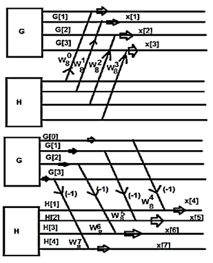
W84 = -1
W8 5 = - W 81
W86 = - W82
W87 = - W83
G(0) – H(0) = x(4)
G(1) - W 81 H(1) = x(5)
G(2) - W82 H(2) = x(6)
G(3) - W83 H(3) = x(7)
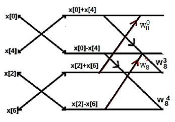
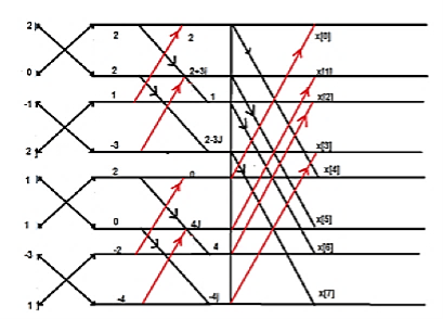
Consider the sequence x[n]={ 2,1,-1,-3,0,1,2,1}. Calculate the FFT.
Arrange the sequence as x(0) x(4) x(2) x(6) x(1) x(5) x(3) x(7)
Since N=8 find the values W8 0 to W 87
Apply the butterfly diagram to obtain the values.
Decimation in Frequency FFT
Apart from time sequence, an N-point sequence can also be represented in frequency. Let us take a four-point sequence to understand it better.
Let the sequence be x[0],x[1],x[2],x[3]………..x[7]
Mathematically, this sequence can be written as;
X(k) =  WN n-k where k=0,1……….. N-1.
Now let us make one group of sequence number 0 to 3 and another group of sequence 4 to 7. Now, mathematically this can be shown as
=  WN nk +
  WN nk
WN nk
Let us replace n by r, where r = 0, 1 , 2….N/2−1.
=  W N/2 nr
We take the first four points x[0],x[1],x[2],x[3] initially, and try to represent them mathematically as follows –
 W 8 nk +
  W8 (n+4) k
=  +
+  W8 (n+4) k
=  + {
+ {  W8 (4) k } W8 nk
X[0] =  + X[n+4]
X[1] =  + X[n+4]) W8 nk
= X(0) – X(4) + (x[1] – X[5]) W8 1 + ( X[2] – X[6] )W82 + X(3) – X(7) W8 3
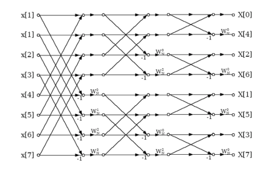
Fig 9 DIF –FFT Algorithm
Find the DIF –FFT of the sequence x(n)= { 1,-1,-1,1,1,1,-1} using Dif-FFT algorithm.
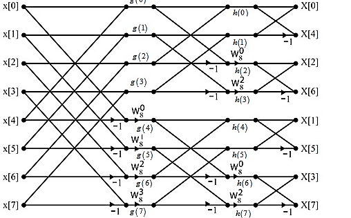
X(0)= 20 X(4) =0
X(1) = -5.828- j2.414 X(5) = -0.1716 + j 0.4141
X(2) = 0 X(6) = 0
X(3) = -0.171 – j 0.4142 X(7) = -5.8284 + j2.4142
References:
- Digital Signal Processing – Principles, Algorithms and Applications by J. G. Proakis and D. G. Manolakis, Pearson.
- Digital Signal Processing: Tarun Kumar Rawat, Oxford University Press.
- Digital Signal Processing – S. Salivahan, A. Vallavraj and C. Gnanapriya, Tata McGrawHill.
- Digital Signal Processing – Manson H. Hayes (Schaum’s Outlines) Adapted by Subrata Bhattacharya, Tata McGraw Hill.
- Digital Signal Processing - Dr. Shalia D. Apte, Willey Publication

