UNIT-2
First order ordinary differential equations
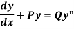
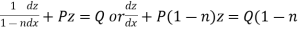
A differential equation of the form

Is called linear differential equation.
It is also called Leibnitz’s linear equation.
Here P and Q are the function of x
Working rule
(1)Convert the equation to the standard form 
(2) Find the integrating factor.
(3) Then the solution will be y(I.F) = 
Example-1: Solve-
Sol. We can write the given equation as-
So that-
I.F. = 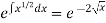
The solution of equation (1) will be-
Or
Or
Or
Example-2: Solve-

Sol.
We can write the equation as-
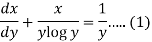
We see that it is a Leibnitz’s equation in x-
So that-
Therefore the solution of equation (1) will be-
Or
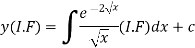
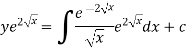
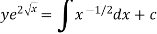
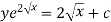
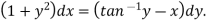
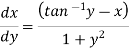
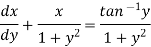
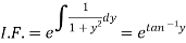
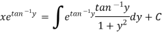
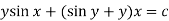
Example-3: Solve sin x 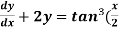 )
)
Solution: here we have,
Sin x  )
)
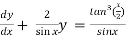 which is the linear form,
Now,
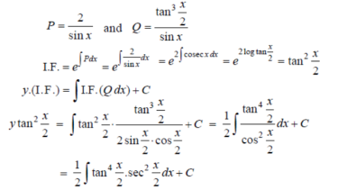
Put tan so that
  sec²
sec² dx = dt, we get
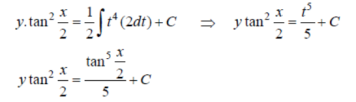
Which is the required solution.
Bernoulli’s equation-
The equation
Is reducible to the Leibnitz’s linear equation and is usually called Bernoulli’s equation.
Working procedure to solve the Bernoulli’s linear equation-
Divide both sides of the equation -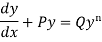
By , so that
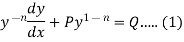
Put  so that
Then equation (1) becomes-
 )
)
Here we see that it is a Leibnitz’s linear equations which can be solved easily.
Example: Solve
Sol.
We can write the equation as-
On dividing by  , we get-
Put  so that
Equation (1) becomes,
Here,
Therefore the solution is-
Or
Now put 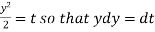
Integrate by parts-
Or
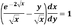
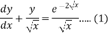
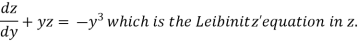
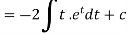
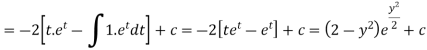
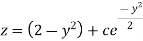
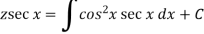
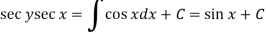
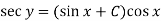
Example: Solve 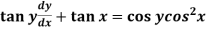
Sol. Here given,
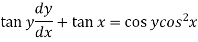
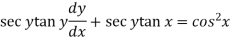
Now let z = sec y, so that dz/dx = sec y tan y dy/dx
Then the equation becomes-
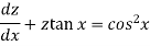
Here,
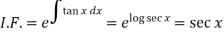
Then the solution will be-
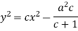
Example: Solve- 
Sol. Here given-
We can re-write this as-
Which is a linear differential equation-
The solution will be-
Put 

Definition-
An exact differential equation is formed by differentiating its solution directly without any other process,
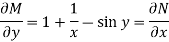
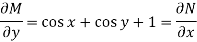
Is called an exact differential equation if it satisfies the following condition-

Here  is the differential co-efficient of M with respect to y keeping x constant and
  is the differential co-efficient of N with respect to x keeping y constant.
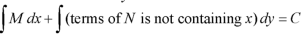
Step by step method to solve an exact differential equation-
1. Integrate M w.r.t. x keeping y constant.
2. Integrate with respect to y, those terms of N which do not contain x.
3. Add the above two results as below-

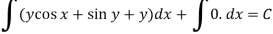
Example-1: Solve 
Sol.
Here M =  and N =
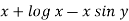
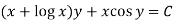
Then the equation is exact and its solution is-
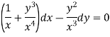
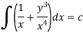
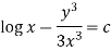
Example-2: Solve-
Sol. We can write the equation as below-

Here M =  and N =
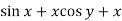
So that-
The equation is exact and its solution will be-
Or
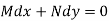
Example-3: Determine whether the differential function ydx –xdy = 0 is exact or not.
Solution. Here the equation is the form of M(x , y)dx + N(x , y)dy = 0
But, we will check for exactness,


These are not equal results, so we can say that the given diff. Eq. Is not exact.
Equation reducible to exact form-
1. If M dx + N dy = 0 be an homogenous equation in x and y, then 1/ (Mx + Ny) is an integrating factor.
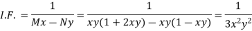
Example: Solve-

Sol.
We can write the given equation as-

Here,
M = 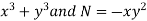
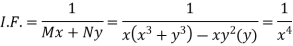
Multiply equation (1) by  we get-
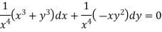
This is an exact differential equation-
2. I.F. For an equation of the type 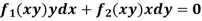
IF the equation Mdx + Ndy = 0 be this form, then 1/(Mx – Ny) is an integrating factor.
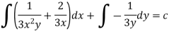
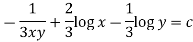
Example: Solve-

Sol.
Here we have-
Now divide by xy, we get-


Multiply (1) by  , we get-
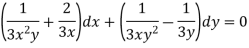
Which is an exact differential equation-
3. In the equation M dx + N dy = 0,
(i) If  be a function of x only = f(x), then
  is an integrating factor.
(ii) If  be a function of y only = F(x), then
  is an integrating factor.
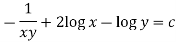
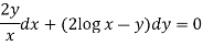
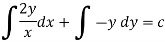
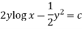
Example: Solve-

Sol.
Here given,

M = 2y and N = 2x log x - xy
Then-
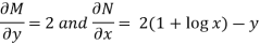
Here,
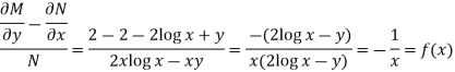
Then,
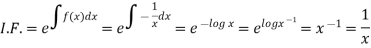
Now multiplying equation (1) by 1/x, we get-
4. For the following type of equation-

An I.F. Is 
Where-
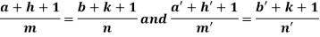
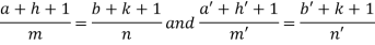
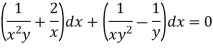
Example: Solve-

Sol.
We can write the equation as below-

Now comparing with-

We get-
a = b = 1, m = n = 1, a’ = b’ = 2, m’ = 2, n’ = -1
I.F. = 
Where-
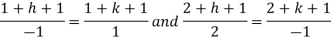
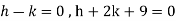
On solving we get-
h = k = -3

Multiply the equation by  , we get-
It is an exact equation.
So that the solution is-

Equation solvable for p-
Example- Solve-

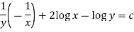
Sol. Here we have-

Or


On integrating, we get-
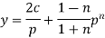
Equation solvable for y-
Steps-
First- differentiate the given equation w.r.t. x.
Second- Eliminate p from the given equation, then the eliminant is the required solution.
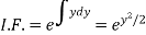
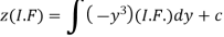
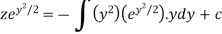
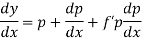
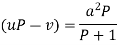
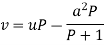
Example: Solve 
Sol.
Here we have-
Now differentiate it with respect to x, we get-
Or
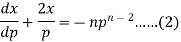
This is the Leibnitz’s linear equation in x and p, here
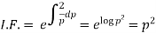
Then the solution of (2) is-
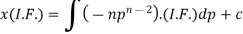
Or
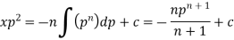
Or

Put this value of x in (1), we get
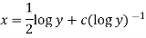
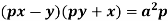
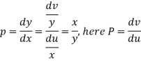
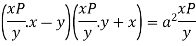
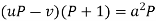
Equation solvable for x-
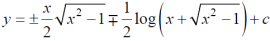
Example: Solve-
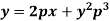
Sol. Here we have-
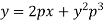
On solving for x, it becomes-

Differentiating w.r.t. y, we get-
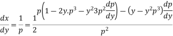
Or
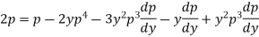
On solving it becomes
Which gives-

Or

On integrating

Thus eliminating from the given equation and (1), we get
Which is the required solution.
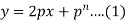
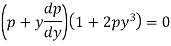
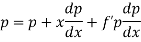
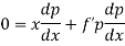
Clairaut’s equation-
An equation
y = px + f(p) ...... (2)
Is known as Clairaut’s equation.
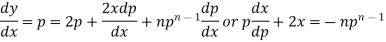
Differentiating (1) w.r.t. x, we get-
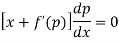

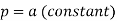
Put the value of p in (1) we get-
y = ax + f(a)
Which is the required solution.
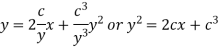
Example: Solve-
Sol.
Put 
So that-
Then the given equation becomes-
Or
Or
Which is the Clairaut’s form.
Its solution is-

i.e.